Bosons in an Optical Lattice

Bandstructure of an homogeneous optical lattice

Theory

At this first moment, we shall look at the simplest case, i.e. a single particle of mass $m$ which experiences a periodic potential:

where $V_0^{x_\alpha}$ is the lattice depth in units of the recoil energy $E_r^\alpha = \frac{\hbar^2}{2m} \left( \frac{2\pi}{\lambda_\alpha} \right)^2$ and lengths are in units of the lattice spacing $\frac{\lambda_\alpha}{2}$.

The quantum mechanical behaviour of the single particle follows:

which is clearly separable to say the $x$-component:

where $k_x = 0, \frac{1}{L_x} ,\cdots \frac{L_x-1}{L_x}$.

In the plane wave basis:

We arrive at a tridiagonal diagonalization problem:

The wannier function is defined as:

and from there, one can calculate the onsite interaction:

After a little bit of algebra, we arrive at the hopping strength:

Finally, the Fourier transform of the wannier function is:

Implementation in Python

The script tutorials/optical-lattice-01-bandstructure/bandstructure.py evaluates these formulas: for each direction it diagonalizes the tridiagonal problem above for all $k_x$, obtains $t$ from the band energies $\epsilon_{k_x}$, and integrates $|w(x)|^4$ to obtain $U$. Run the following from that directory:

import numpy as np
import bandstructure

V0   = np.array([8., 8., 8.])        # lattice depth in recoil energies
wlen = np.array([843., 843., 843.])  # laser wavelength in nanometer
a    = 114.8                         # s-wave scattering length in bohr radius
m    = 86.99                         # mass in atomic mass unit
L    = 200                           # lattice size (along 1 direction)

t, U = bandstructure.hubbard_parameters(V0, wlen, a, m, L)

print(t)        # t in nK:  [4.77051684 4.77051684 4.77051684]
print(U)        # U in nK:  38.70187649673881
print(U / t)    # U/t:      [8.11272191 8.11272191 8.11272191]

Bosons in an optical lattice trap

Boson Hubbard model

Hamiltonian

Bosons in an optical lattice trap can be effectively described by the single band boson Hubbard model:

with hopping strength $t$, onsite interaction strength $U$, and chemical potential $\mu$ at finite temperature $T$ via the directed-loop stochastic series expansion (SSE) quantum Monte Carlo code dirloop_sse. Here, $\hat{b}$ ($\hat{b}^+$) is the annihilation (creation) operator, and $\hat{n}_i$ being the number operator at site $i$. Bosons in an optical lattice are confined in a 3D parabolic trapping potential:

due to the gaussian beam waists as well as other sources of trapping.

Finite temperature

At finite temperature $T$, the physics is essentially captured by the partition function:

and physical quantities such as the local density:

for some configuration $\mathcal{C}$ in the complete configuration space, with inverse temperature $\beta = 1/T$ . Here, the units will be cleverly normalized later on.

Implementation in Python

The script tutorials/optical-lattice-02-density-profile/density_profile.py simulates this model on a $9^3$ lattice with dirloop_sse and plots the local density $\langle n_i \rangle$. It uses $U/t = 8.11$ from the band-structure example above, temperature $T = t$, and an isotropic trap $K_x = K_y = K_z = 0.65\,t$ centered on the lattice. The trap enters through a site-dependent chemical potential on the inhomogeneous simple cubic lattice:

import numpy as np
import pyalps

L = 9
K = 0.65                                        # trap curvature V_T = K r^2, in units of t
c = (L - 1) / 2.

parms = [{
    'LATTICE' : 'inhomogeneous simple cubic lattice',
    'L'       : L,
    'MODEL'   : 'boson Hubbard',
    'Nmax'    : 4,
    't'       : 1.,
    'U'       : 8.11,
    'mu'      : '4.05 - %g*((x-%g)*(x-%g) + (y-%g)*(y-%g) + (z-%g)*(z-%g))' % ((K,) + (c,) * 6),
    'T'       : 1.,
    'THERMALIZATION' : 1000,
    'SWEEPS'         : 5000,
    'MEASURE_LOCAL[Local Density]' : 'n',
}]

input_file = pyalps.writeInputFiles('parm_trap', parms)
pyalps.runApplication('dirloop_sse', input_file)

data = pyalps.loadMeasurements(pyalps.getResultFiles(prefix='parm_trap'), 'Local Density')[0][0]
n = np.asarray(data.y.mean).reshape(L, L, L)
print('Total number of bosons: %.2f' % n.sum())
print('Density at the trap center: %.3f' % n[L // 2, L // 2, L // 2])

The full script also plots a cut through the trap center and the density in the center layer:

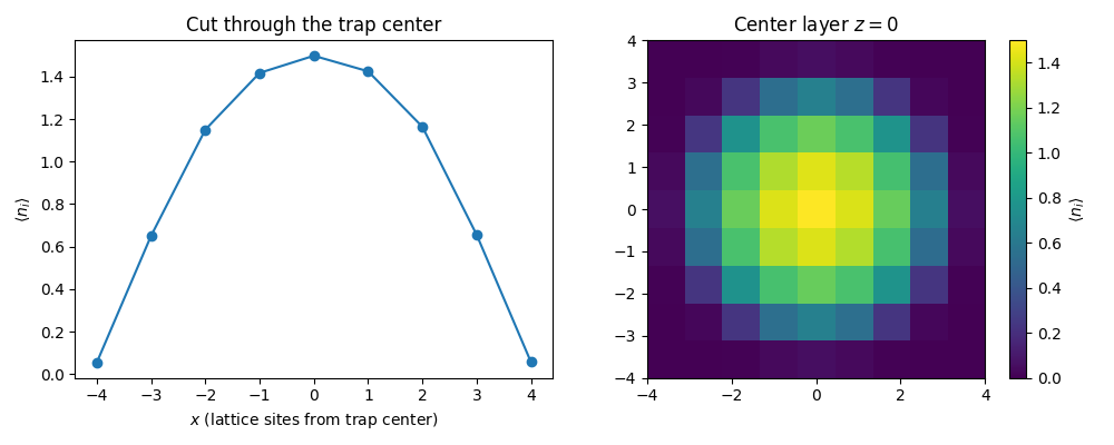
The lattice is kept small so the example runs in a few minutes, which means it still sits inside the cloud: the density falls off toward the edges but does not quite vanish there. A bigger lattice lets the density drop closer to zero at the edges.

Contributors

• Ping Nang Ma
• Matthias Troyer