Exact Diagonaliztion
As an example of the sparse exact diagonalization method, we will obtain the triplet gap as a function of system size for the spin chain model.
First step is import required packages.
import pyalps
import numpy as np
import matplotlib.pyplot as plt
import pyalps.plot
import pyalps.fit_wrapper as fw
Then we prepare each set of input parameters and write them into the format ALPS expects.
parms = []
for l in [4, 6, 8, 10, 12, 14, 16]:
  for sz in [0, 1]:
      parms.append(
        {
          'LATTICE'                   : "chain lattice",
          'MODEL'                     : "spin",
          'local_S'                   : 1,
          'J'                         : 1,
          'L'                         : l,
          'CONSERVED_QUANTUMNUMBERS'  : 'Sz',
          'Sz_total'                  : sz
        }
      )

#write the input file and run the simulation
input_file = pyalps.writeInputFiles('parm2a',parms)
Then we run sparsediag for each set of parameters:
res = pyalps.runApplication('sparsediag',input_file)We then load measurements for all states:
data = pyalps.loadSpectra(pyalps.getResultFiles(prefix='parm2a'))And extract the ground state energies over all momenta for every simulation.
lengths = []
min_energies = {}
for sim in data:
l = int(sim[0].props['L'])
if l not in lengths: lengths.append(l)
sz = int(sim[0].props['Sz_total'])
all_energies = []
for sec in sim:
all_energies += list(sec.y)
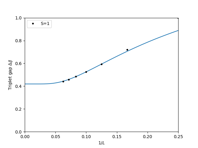
min_energies[(l,sz)]= np.min(all_energies)Finally, we make a plot of the triplet gap as a function of system size.
gapplot = pyalps.DataSet()
gapplot.x = 1./np.sort(lengths)
gapplot.y = [min_energies[(l,1)] -min_energies[(l,0)] for l in np.sort(lengths)]
gapplot.props['xlabel']='$1/L$'
gapplot.props['ylabel']='Triplet gap $\Delta/J$'
gapplot.props['label']='S=1'
gapplot.props['line']='.'

plt.figure()
pyalps.plot.plot(gapplot)
plt.legend()
plt.xlim(0,0.25)
plt.ylim(0,1.0)

pars = [fw.Parameter(0.411), fw.Parameter(1000), fw.Parameter(1)]
f = lambda self, x, p: p[0]()+p[1]()*np.exp(-x/p[2]())
# we fit only a range from 8 to 16
fw.fit(None, f, pars, np.array(gapplot.y)[2:], np.sort(lengths)[2:])

x = np.linspace(0.0001, 1./min(lengths), 100)
plt.plot(x, f(None, 1/x, pars))

plt.show()
The final result should look like this: