Classical Monte Carlo Simulations

The 2D Ising model is one of the most important models in statistical mechanics. It describes spins on a square lattice that can point either up or down, with ferromagnetic coupling $J > 0$ between nearest neighbors (using spinmc’s default classical sign convention, where positive $J$ favors parallel spins). Onsager showed in 1944 that it has an exact solution with a phase transition at $T_c = 2J / \ln(1 + \sqrt{2}) \approx 2.269\, J/k_B$: below $T_c$ the spins order spontaneously, above $T_c$ thermal fluctuations destroy that order.

This tutorial simulates that phase transition using ALPS. It is a good first example because the physics is well understood and the result is easy to check.

Import packages

pyalps provides the simulation framework and analysis tools. matplotlib and pyalps.plot are used for visualization.

import pyalps
import matplotlib.pyplot as plt
import pyalps.plot

Set up parameters

We simulate square lattices of three sizes — $4\times 4$, $8\times 8$, and $16\times 16$ — over a range of temperatures. Running multiple system sizes lets us see how the transition sharpens as the system grows toward the thermodynamic limit.

The parameters for each run are collected in a list of dictionaries:

parms = []
for l in [4, 8, 16]:
    for t in [5.0, 4.5, 4.0, 3.5, 3.0, 2.9, 2.8, 2.7]:
        parms.append({
            'LATTICE'        : "square lattice",
            'T'              : t,
            'J'              : 1,
            'THERMALIZATION' : 1000,
            'SWEEPS'         : 400000,
            'UPDATE'         : "cluster",
            'MODEL'          : "Ising",
            'L'              : l,
        })
    for t in [2.6, 2.5, 2.4, 2.3, 2.2, 2.1, 2.0, 1.9, 1.8, 1.7, 1.6, 1.5, 1.2]:
        parms.append({
            'LATTICE'        : "square lattice",
            'T'              : t,
            'J'              : 1,
            'THERMALIZATION' : 1000,
            'SWEEPS'         : 40000,
            'UPDATE'         : "cluster",
            'MODEL'          : "Ising",
            'L'              : l,
        })

A few key parameters to understand:

• THERMALIZATION: the number of Monte Carlo sweeps discarded at the start of each run to let the system reach equilibrium before measurements begin.
• SWEEPS: the number of measurement sweeps after thermalization. More sweeps reduce statistical noise. We use more sweeps ($400\,000$) at high temperatures, where the correlation length is short and individual sweeps are cheap, and fewer ($40\,000$) near and below $T_c$ where cluster updates are larger.
• UPDATE: "cluster": selects the Wolff cluster algorithm instead of single-spin-flip Metropolis. Near $T_c$, single-spin-flip updates suffer from critical slowing down — the simulation becomes very inefficient because the spin correlation length diverges. The cluster algorithm flips whole correlated domains at once and largely avoids this problem.
• L: the linear system size. A lattice with L = 8 has $8 \times 8 = 64$ spins.

The temperature grid is coarser far from $T_c$ and finer in the range $1.2$–$2.7$ where the interesting physics happens.

Run the simulation

writeInputFiles converts the parameter list into the XML input format that ALPS expects and writes it to disk. runApplication then launches the spinmc executable. The Tmin=5 argument tells ALPS to use at least 5 seconds of CPU time per run.

input_file = pyalps.writeInputFiles('parm7a', parms)
pyalps.runApplication('spinmc', input_file, Tmin=5)

Evaluate and plot

evaluateSpinMC post-processes the raw simulation output to compute derived quantities such as the magnetic susceptibility and the Binder cumulant. loadMeasurements reads the results back into Python, and collectXY organizes them as curves of $|m|$ vs. $T$, one curve per system size.

pyalps.evaluateSpinMC(pyalps.getResultFiles(prefix='parm7a'))

# load the magnetization as a function of temperature
data = pyalps.loadMeasurements(pyalps.getResultFiles(prefix='parm7a'), ['|Magnetization|'])
magnetization_abs = pyalps.collectXY(data, x='T', y='|Magnetization|', foreach=['L'])

# plot
plt.figure()
pyalps.plot.plot(magnetization_abs)
plt.xlabel('Temperature $T$')
plt.ylabel('Magnetization $|m|$')
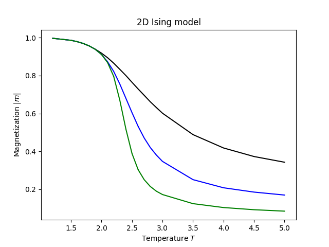
plt.title('2D Ising model')
plt.show()

The magnetization drops from nearly 1 at low temperature to 0 above $T_c \approx 2.269$. For small systems the transition is rounded by finite-size effects; it sharpens and shifts toward the exact $T_c$ as $L$ increases:

Walkthrough Video