DMRG

Density Matrix Renormalization Group

This tutorial assumes that pyalps is already installed. If you have not set it up yet, see the Getting Started guide.

What is DMRG?

The Density Matrix Renormalization Group (DMRG) was introduced by Steven White in 1992 and quickly became the method of choice for one-dimensional quantum lattice models. DMRG finds the ground state variationally within the family of matrix product states (MPS): wave functions of the form

|\psi\rangle = \sum_{s_1, \ldots, s_L} A_1^{s_1} A_2^{s_2} \cdots A_L^{s_L} \, |s_1 s_2 \cdots s_L\rangle,

where each $A_i^{s_i}$ is a matrix of dimension at most $m \times m$ . The integer $m$ — called the bond dimension — controls the accuracy of the approximation: $m = 1$ is a product state, and increasing $m$ captures more quantum entanglement.

Why does this work so well in 1D? Gapped ground states of local Hamiltonians satisfy an area law: the entanglement entropy of any contiguous block of sites is bounded by a constant independent of block size. This means the exact ground state can be well approximated by an MPS with a fixed, moderate $m$ . For the $S = 1/2$ Heisenberg chain (which is gapless), the entanglement entropy grows only logarithmically, so $m \sim 100$ – $1000$ is typically sufficient.

DMRG optimizes the matrices $A_i$ by sweeping: it starts from one end of the chain, optimizes the matrices at each site in turn while holding all others fixed, then sweeps back from the other end, repeating until convergence. Each optimization step is a small eigenvalue problem — far cheaper than the full diagonalization that ED requires. The cost of a DMRG sweep scales as $O(L m^3 d)$ , where $d$ is the local Hilbert space dimension, versus $O(d^L)$ for ED. For $L = 32$ and $d = 2$ , ED would require $2^{32} \approx 4$ billion states; DMRG with $m = 100$ is entirely routine.

Why open boundary conditions? DMRG is far more efficient on chains with open boundaries (OBC) than with periodic boundary conditions (PBC). With PBC, the entanglement structure wraps around the chain, roughly doubling the effective bond dimension needed for the same accuracy. OBC is therefore the standard choice for DMRG calculations.

The physical model

We study the $S = 1/2$ antiferromagnetic Heisenberg chain,

H = J \sum_{i=1}^{L-1} \mathbf{S}_i \cdot \mathbf{S}_{i+1}, \quad J > 0,

on $L = 32$ sites with open boundary conditions. Unlike the $S = 1$ chain (which has the Haldane gap), the $S = 1/2$ chain is gapless: its low-energy spectrum forms a Tomonaga-Luttinger liquid (TLL) with power-law correlations. Its exact ground-state energy per bond in the thermodynamic limit is given by the Bethe ansatz:

e_0 = \frac{1}{4} - \ln 2 \approx -0.4431\,J \quad \text{per bond}.

This is one of the most-studied benchmark systems in computational quantum physics and an ideal starting point for learning DMRG.

Running the simulation

The entire setup, run, and analysis fits in a single Python script:

import pyalps
import numpy as np
import matplotlib.pyplot as plt
import pyalps.plot

parms = [ {
        'LATTICE'                  : "open chain lattice",   # open boundary conditions (better for DMRG)
        'MODEL'                    : "spin",
        'CONSERVED_QUANTUMNUMBERS' : 'N,Sz',                 # exploit N and Sz conservation to block-diagonalize
        'Sz_total'                 : 0,                      # target the Sz=0 sector (ground state)
        'J'                        : 1,                      # antiferromagnetic exchange
        'SWEEPS'                   : 4,                      # number of DMRG sweeps (left→right→left = 1 sweep)
        'NUMBER_EIGENVALUES'       : 1,                      # find only the ground state
        'L'                        : 32,                     # chain length
        'MAXSTATES'                : 100                     # bond dimension m (key accuracy parameter)
       } ]

input_file = pyalps.writeInputFiles('parm_spin_one_half', parms)
res = pyalps.runApplication('dmrg', input_file, writexml=True)

Parameter notes

MAXSTATES is the most important accuracy parameter. It sets the maximum bond dimension $m$ . Increasing it improves accuracy at the cost of compute time (which scales as $m^3$ ). For this 32-site benchmark, $m = 100$ gives a truncation error well below $10^{-6}$ .
SWEEPS is the number of full left-to-right-and-back sweeps. Four sweeps is enough to demonstrate convergence here; production calculations often use 10–20 sweeps, or sweep until the energy change per sweep falls below a threshold.
CONSERVED_QUANTUMNUMBERS: 'N,Sz' tells DMRG to exploit both total particle number $N$ and total magnetization $S_z$ as good quantum numbers, block-diagonalizing the MPS matrices. This makes the calculation faster and more numerically stable.
NUMBER_EIGENVALUES: 1 targets only the ground state. Increasing this allows DMRG to target the lowest few eigenstates simultaneously, at additional cost.

Loading ground state observables

After the simulation, loadEigenstateMeasurements retrieves all observables measured by the DMRG code — energy, magnetization, correlation functions, and any other quantities ALPS computed for the final converged ground state:

data = pyalps.loadEigenstateMeasurements(pyalps.getResultFiles(prefix='parm_spin_one_half'))

for s in data[0]:
    print(s.props['observable'], ' : ', s.y[0])

Each element s in data[0] corresponds to one observable. s.props['observable'] is its name (e.g., 'Energy', 'Magnetization') and s.y[0] is its value. The ground-state energy should be close to $E_0 \approx -14.3\,J$ for this 32-site open chain.

Loading iteration history

To understand how the algorithm converged, we load per-sweep measurements:

itr = pyalps.loadMeasurements(pyalps.getResultFiles(prefix='parm_spin_one_half'),
                               what=['Iteration Energy', 'Iteration Truncation Error'])

itr[0][0] contains the energy recorded at each half-sweep; itr[0][1] contains the truncation error at each step. The truncation error is the sum of the discarded eigenvalues of the reduced density matrix — the weight in the exact ground state that the MPS with $m$ states cannot represent. A well-converged calculation should reach a truncation error below $10^{-6}$ ; for $m = 100$ on this system, values around $10^{-8}$ – $10^{-7}$ are typical.

Plotting convergence

plt.figure()
pyalps.plot.plot(itr[0][0])
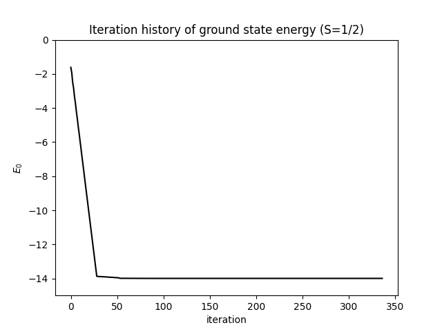
plt.title('Iteration history of ground state energy (S=1/2)')
plt.ylim(-15, 0)
plt.ylabel('$E_0$')
plt.xlabel('Iteration')

plt.figure()
pyalps.plot.plot(itr[0][1])
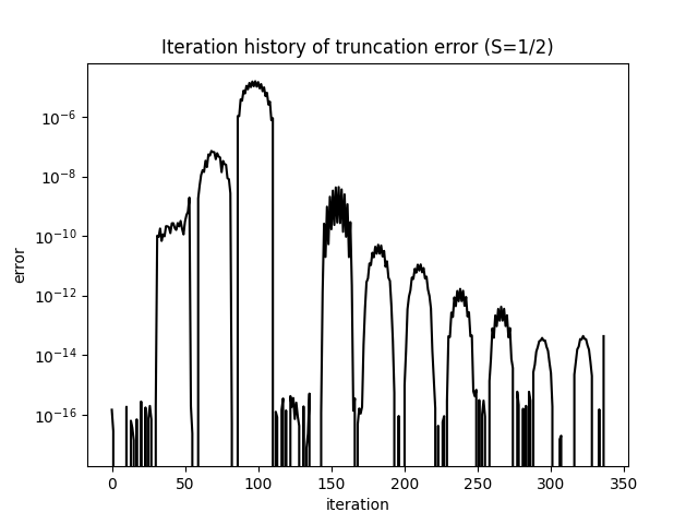
plt.title('Iteration history of truncation error (S=1/2)')
plt.yscale('log')
plt.ylabel('Truncation error')
plt.xlabel('Iteration')

plt.show()

Results

The energy converges rapidly to a plateau within the first few sweeps. The plot below shows the energy as a function of iteration number — it stabilizes well before the final sweep:

Ground state energy convergence over DMRG iterations

The truncation error decays monotonically on a logarithmic scale, reflecting the improving quality of the MPS approximation with each sweep:

Truncation error decay over DMRG iterations (log scale)

Once both curves have flattened, the calculation is converged. To improve accuracy further, increase MAXSTATES and verify that the energy and truncation error change negligibly.

CT-HYB Exact Diagonalization