Exact Diagonalization

What is exact diagonalization?

Exact diagonalization (ED) is the most direct approach to solving a quantum many-body problem: build the Hamiltonian matrix explicitly in a basis of many-body states, then find its eigenvalues and eigenvectors. The result is numerically exact — no approximations, no sign problem, no sampling error. The catch is cost: for a spin-$S$ chain of $L$ sites, the Hilbert space has dimension $(2S+1)^L$, which grows exponentially. For $S=1$ this means $3^{16} \approx 43$ million states for $L = 16$, and $3^{20} \approx 3.5$ billion for $L = 20$ — already at the edge of what is tractable even on large computers.

The ALPS sparsediag code addresses this with sparse diagonalization via the Lanczos algorithm: instead of diagonalizing the full matrix, it builds a small Krylov subspace from repeated matrix-vector products $H|\psi\rangle$ and extracts the lowest few eigenvalues from it. This is practical because the Heisenberg Hamiltonian is extremely sparse — each basis state is connected to only $O(L)$ others (one per bond), so each matrix-vector product costs $O(L \cdot \dim)$ rather than $O(\dim^2)$.

ED complements QMC: it gives exact ground-state and low-energy spectra at zero temperature, works for any model regardless of sign problems, but is limited to system sizes accessible by Lanczos ($L \lesssim 20$ for $S=1$).

The physical model: the S=1 Heisenberg chain

This tutorial studies the antiferromagnetic Heisenberg model on a one-dimensional chain,

where each $\mathbf{S}_i$ is a spin-1 operator. This model describes a chain of magnetic moments with antiferromagnetic nearest-neighbor exchange.

The Haldane conjecture

In 1983, Duncan Haldane made a surprising prediction: the ground state of integer-spin antiferromagnetic chains ($S = 1, 2, \ldots$) is gapped — there is a finite energy cost $\Delta$ to create any excitation above the ground state. Half-integer chains ($S = 1/2, 3/2, \ldots$), by contrast, are gapless, with a continuous spectrum of low-energy excitations all the way down to zero energy.

This was unexpected because classical intuition and simple mean-field arguments suggest both cases should behave similarly. The distinction arises from a topological contribution in the quantum field theory description that is present for half-integer but absent for integer spin. Haldane’s conjecture was initially controversial, but it has since been confirmed numerically to high precision and experimentally in materials such as Ni(C$_2$H$_8$N$_2$)$_2$NO$_2$(ClO$_4$) (NENP).

For the $S = 1$ chain, the gap converges to

in the thermodynamic limit ($L \to \infty$). On a finite chain of length $L$, the apparent gap is larger and closes exponentially toward the thermodynamic value:

where $\xi \approx 6$ is the correlation length of the Haldane phase. Because $\xi$ is not small, chains up to $L = 16$ still show significant finite-size corrections — this is why a careful extrapolation is needed.

Strategy

We will:

1. Run sparsediag on chains of length $L \in \{4, 6, 8, 10, 12, 14, 16\}$.
2. For each $L$, compute the lowest energy in the $S_z = 0$ sector (singlet ground state) and the $S_z = 1$ sector (lowest triplet state).
3. Form the gap $\Delta(L) = E_0(S_z=1,L) - E_0(S_z=0,L)$.
4. Fit the exponential finite-size formula and extract $\Delta$.

Imports

import pyalps
import numpy as np
import matplotlib.pyplot as plt
import pyalps.plot
import pyalps.fit_wrapper as fw

Quantum number sectors

Before looking at the code, it is worth understanding why we run two separate diagonalizations per chain length — one with Sz_total=0 and one with Sz_total=1.

The Heisenberg Hamiltonian commutes with the total magnetization $S_z^{\text{total}} = \sum_i S_z^i$, meaning total $S_z$ is conserved: $[H, S_z^{\text{total}}] = 0$. The full Hilbert space therefore block-diagonalizes into independent sectors labelled by $S_z^{\text{total}} = -SL, \ldots, SL$. We can diagonalize each block independently.

This is the key to making ED tractable. For $L = 16$, $S = 1$, the full Hilbert space has dimension $3^{16} \approx 43$ million; the $S_z = 0$ sector has dimension roughly $14$ million — smaller, but crucially, ALPS also exploits translational symmetry and parity, reducing the effective dimension by another factor of $2L$. Working in sectors rather than the full space is essential.

The singlet ground state of the antiferromagnet lies in $S_z = 0$. The lowest triplet excited state — the first state with total spin 1 — appears as the ground state of the $S_z = 1$ sector. Their energy difference is the triplet gap.

Parameters and input files

parms = []
for l in [4, 6, 8, 10, 12, 14, 16]:
    for sz in [0, 1]:
        parms.append(
          {
            'LATTICE'                  : "chain lattice",
            'MODEL'                    : "spin",
            'local_S'                  : 1,               # S=1 spin chain
            'J'                        : 1,               # antiferromagnetic exchange (sets energy scale)
            'L'                        : l,               # chain length
            'CONSERVED_QUANTUMNUMBERS' : 'Sz',            # tell ALPS to block-diagonalize in Sz
            'Sz_total'                 : sz               # target sector (0=singlet, 1=triplet)
          }
        )

input_file = pyalps.writeInputFiles('parm2a', parms)

writeInputFiles creates the XML input files in the ALPS format that sparsediag reads. The prefix 'parm2a' is used to name the output files.

Running the solver

res = pyalps.runApplication('sparsediag', input_file)

sparsediag runs the Lanczos algorithm on each parameter set. For each combination of $(L, S_z)$, it further block-diagonalizes within the $S_z$ sector using translational symmetry — so it actually solves one smaller matrix per lattice momentum $k = 0, \frac{2\pi}{L}, \ldots, \frac{2\pi(L-1)}{L}$. The output is stored in HDF5 files named after the prefix.

Loading results and understanding the data structure

data = pyalps.loadSpectra(pyalps.getResultFiles(prefix='parm2a'))

data is a list of simulations, one per parameter set. Each element sim in data is itself a list of DataSet objects — one per lattice-momentum subsector $k$ within the chosen $S_z$ sector. Each DataSet carries:

• sec.props: the parameters for this run (including 'L', 'Sz_total', 'TOTAL_MOMENTUM').
• sec.y: a NumPy array of eigenvalues found in this $k$-subsector.

Extracting the gap

The ground state in each $S_z$ sector can have any lattice momentum, so we collect all eigenvalues across all $k$-subsectors and take the global minimum:

lengths      = []
min_energies = {}
for sim in data:
    l  = int(sim[0].props['L'])
    if l not in lengths: lengths.append(l)
    sz = int(sim[0].props['Sz_total'])
    all_energies = []
    for sec in sim:          # loop over k-subsectors within this (L, Sz) run
        all_energies += list(sec.y)
    min_energies[(l, sz)] = np.min(all_energies)

After this loop, min_energies[(l, 0)] is the ground-state energy in the singlet sector and min_energies[(l, 1)] is the ground-state energy in the triplet sector, for each chain length $l$.

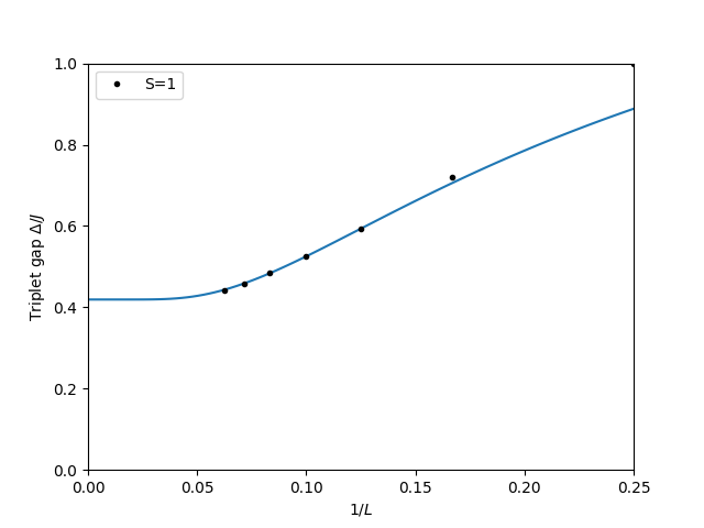
Finite-size extrapolation

The gap at each finite size is:

We plot it against $1/L$ and fit the exponential finite-size correction:

Note that the plot uses $1/L$ as the $x$-axis (so the thermodynamic limit is at $x = 0$), but the fit function f is written in terms of $L$ and called with 1/x. The fw.Parameter objects hold the fit parameters; after fw.fit runs, p[0]() retrieves the fitted value of $\Delta$, p[1]() gives $A$, and p[2]() gives $\xi$.

We fit only $L \geq 8$ (index [2:] skips $L = 4$ and $L = 6$) to avoid the largest corrections-to-scaling that occur on the smallest chains, where the chain length is not much larger than the lattice spacing:

gapplot = pyalps.DataSet()
gapplot.x = 1./np.sort(lengths)
gapplot.y = [min_energies[(l,1)] - min_energies[(l,0)] for l in np.sort(lengths)]
gapplot.props['xlabel'] = '$1/L$'
gapplot.props['ylabel'] = 'Triplet gap $\Delta/J$'
gapplot.props['label']  = 'S=1'
gapplot.props['line']   = '.'

plt.figure()
pyalps.plot.plot(gapplot)
plt.legend()
plt.xlim(0, 0.25)
plt.ylim(0, 1.0)

# Initial guesses: Delta~0.411 (known Haldane gap), A~1000, xi~6
pars = [fw.Parameter(0.411), fw.Parameter(1000), fw.Parameter(6)]
f = lambda self, x, p: p[0]() + p[1]()*np.exp(-x/p[2]())
fw.fit(None, f, pars, np.array(gapplot.y)[2:], np.sort(lengths)[2:])  # fit L >= 8

x = np.linspace(0.0001, 1./min(lengths), 100)
plt.plot(x, f(None, 1/x, pars))

plt.show()

Result

The fitted curve extrapolates to the $y$-intercept at $1/L = 0$, giving $\Delta \approx 0.411\,J$ — in good agreement with the best numerical estimates for the Haldane gap (White & Huse, 1993: $\Delta = 0.41048\,J$). This confirms the Haldane phase and validates the ALPS sparsediag solver.

The plot shows the triplet gap decreasing as $L$ grows, with the fitted curve capturing the exponential convergence: