CT-HYB

CT-HYB Impurity Solver

This tutorial assumes that pyalps is already installed. If you have not set it up yet, see the Getting Started guide.

This tutorial demonstrates the continuous-time hybridization-expansion (CT-HYB) quantum Monte Carlo solver — an exact, numerically unbiased method for quantum impurity models, originally introduced by Werner et al. (Phys. Rev. Lett. 97, 076405, 2006). We simulate the Kondo effect: as temperature decreases, conduction electrons screen a magnetic impurity, progressively reducing its effective local moment. The dimensionless effective moment is $4T\chi_{dd}$ , where $\chi_{dd}$ is the local spin susceptibility. At high temperature it approaches 1 (free spin, $S = 1/2$ ); for a non-zero Coulomb interaction $U > 0$ , it decreases toward zero at low temperature, signaling complete Kondo screening. We use a semielliptic density of states as the hybridization function — a standard choice corresponding to the Bethe lattice, commonly encountered in dynamical mean-field theory (DMFT) calculations.

Imports

from pyalps.hdf5 import archive       # HDF5 archive interface
import pyalps.cthyb as cthyb          # CT-HYB impurity solver
import matplotlib.pyplot as plt       # for plotting results
from numpy import exp, log, sqrt, pi  # math utilities

Temperature grid

We generate 11 temperature points between $T_{\min} = 0.05$ and $T_{\max} = 100.0$ , spaced equally on a logarithmic scale to sample both the high-temperature free-spin regime and the low-temperature Kondo-screened regime:

N_T  = 11     # number of temperature points (includes both endpoints)
Tmin = 0.05   # minimum temperature
Tmax = 100.0  # maximum temperature
Tdiv = exp(log(Tmax/Tmin)/(N_T - 1))
T = Tmax
Tvalues = []
for i in range(N_T):
    Tvalues.append(T)
    T /= Tdiv

Simulation parameters

We compare two values of the on-site Coulomb interaction: $U = 0$ (non-interacting reference) and $U = 2$ (interacting, Kondo regime). Key parameters:

N_TAU: Number of imaginary-time grid points $\tau \in [0, \beta]$ . Must be large enough to resolve the lowest temperature; a safe rule of thumb is $N_\tau \geq 5\beta U$ .
runtime: Wall-clock seconds allocated to each solver call. Increase this for production runs to improve statistical accuracy.

Uvalues = [0., 2.]  # on-site Coulomb interaction values
N_TAU   = 1000      # imaginary-time points; at least 5*BETA*U for the lowest temperature
runtime = 5         # solver runtime per temperature point (seconds)

Building the parameter list

For each combination of $U$ and $T$ , we construct a parameter dictionary:

SWEEPS: Upper bound on Monte Carlo moves. In practice, MAX_TIME stops the solver first.
THERMALIZATION: Moves discarded at the start before measurements begin (equilibration).
N_MEAS: A measurement is recorded once every N_MEAS sweeps.
N_ORBITALS: Number of spin-orbital flavors — here 2 for spin-up and spin-down.
MU: Chemical potential. Set to $U/2$ to enforce particle-hole symmetry at half-filling.
BETA: Inverse temperature $\beta = 1/T$ .

values     = [[] for u in Uvalues]
errors     = [[] for u in Uvalues]
parameters = []
for un, u in enumerate(Uvalues):
    for t in Tvalues:
        parameters.append(
         {
           # solver parameters
           'SWEEPS'             : 1000000000,                          # total Monte Carlo moves (capped by MAX_TIME)
           'THERMALIZATION'     : 1000,                                # equilibration moves (discarded)
           'SEED'               : 42,                                  # random number seed
           'N_MEAS'             : 10,                                  # sweeps between measurements
           'N_ORBITALS'         : 2,                                   # spin-orbital flavors (spin-up, spin-down)
           'BASENAME'           : "hyb.param_U%.1f_BETA%.3f"%(u,1/t), # base name for the HDF5 output file
           'MAX_TIME'           : runtime,                             # wall-clock time limit per solver call (seconds)
           'VERBOSE'            : 1,                                   # print solver progress
           'TEXT_OUTPUT'        : 0,                                   # disable human-readable text output
           # file names
           'DELTA'              : "Delta_BETA%.3f.h5"%(1/t),           # hybridization function input file
           'DELTA_IN_HDF5'      : 1,                                   # read hybridization from HDF5
           # physical parameters
           'U'                  : u,                                   # on-site Coulomb repulsion
           'MU'                 : u/2.,                                # chemical potential (half-filling)
           'BETA'               : 1/t,                                 # inverse temperature
           # measurements
           'MEASURE_nnw'        : 1,                                   # density-density correlator on Matsubara frequencies
           'MEASURE_time'       : 0,                                   # disable imaginary-time measurements
           # discretization
           'N_HISTOGRAM_ORDERS' : 50,                                  # max perturbation order for histogram
           'N_TAU'              : N_TAU,                               # imaginary-time points (tau_0=0, tau_{N_TAU}=beta)
           'N_MATSUBARA'        : int(N_TAU/(2*pi)),                   # Matsubara frequency points
           'N_W'                : 1,                                   # bosonic Matsubara points for local susceptibility
           # bookkeeping
           't'                  : 1,                                   # hopping amplitude (sets energy scale)
           'Un'                 : un,                                  # index into Uvalues (for postprocessing)
         }
        )

Hybridization function

The CT-HYB solver requires the hybridization function $\Delta(\tau)$ as input, which encodes the coupling to the conduction-electron bath. We use a semielliptic density of states with half-bandwidth $D = 2t$ , and compute $\Delta(\tau) = t^2 G_0(\tau)$ via a Fourier transform of the non-interacting Green’s function. The high-frequency tail is subtracted before the transform for numerical stability, then added back analytically.

for parms in parameters:
    ar = archive(parms['BASENAME']+'.out.h5', 'a')
    ar['/parameters'] = parms
    del ar
    print("Creating hybridization function...")
    g  = []
    I  = complex(0., 1.)
    mu = 0.0
    for n in range(parms['N_MATSUBARA']):
        w = (2*n+1)*pi/parms['BETA']
        g.append(2.0/(I*w + mu + I*sqrt(4*parms['t']**2 - (I*w+mu)**2)))  # semielliptic Green's function
    delta = []
    for i in range(parms['N_TAU']+1):
        tau   = i*parms['BETA']/parms['N_TAU']
        g0tau = 0.0
        for n in range(parms['N_MATSUBARA']):
            iw     = complex(0.0, (2*n+1)*pi/parms['BETA'])
            g0tau += ((g[n] - 1.0/iw)*exp(-iw*tau)).real  # Fourier transform with tail subtracted
        g0tau *= 2.0/parms['BETA']
        g0tau += -1.0/2.0                                  # add back the tail contribution
        delta.append(parms['t']**2 * g0tau)                # Delta(tau) = t^2 * G0(tau)

    ar = archive(parms['DELTA'], 'w')
    for m in range(parms['N_ORBITALS']):
        ar['/Delta_%i'%m] = delta
    del ar

Running the solver

for parms in parameters:
    cthyb.solve(parms)

Postprocessing and plotting

We extract the density-density correlator $\langle n_\uparrow n_\uparrow \rangle$ , $\langle n_\downarrow n_\downarrow \rangle$ , and $\langle n_\uparrow n_\downarrow \rangle$ at the zeroth bosonic Matsubara frequency to compute the local spin susceptibility $\chi_{dd} = (\langle n_\uparrow n_\uparrow \rangle + \langle n_\downarrow n_\downarrow \rangle - 2\langle n_\uparrow n_\downarrow \rangle)/4$ .

for parms in parameters:
    ar      = archive(parms['BASENAME']+'.out.h5', 'a')
    nn_0_0  = ar['simulation/results/nnw_re_0_0/mean/value']
    nn_1_1  = ar['simulation/results/nnw_re_1_1/mean/value']
    nn_1_0  = ar['simulation/results/nnw_re_1_0/mean/value']
    dnn_0_0 = ar['simulation/results/nnw_re_0_0/mean/error']
    dnn_1_1 = ar['simulation/results/nnw_re_1_1/mean/error']
    dnn_1_0 = ar['simulation/results/nnw_re_1_0/mean/error']

    nn  = nn_0_0 + nn_1_1 - 2*nn_1_0
    dnn = sqrt(dnn_0_0**2 + dnn_1_1**2 + (2*dnn_1_0)**2)

    ar['chi']  = nn/4.
    ar['dchi'] = dnn/4.
    del ar

    T = 1/parms['BETA']
    values[parms['Un']].append(T*nn[0])
    errors[parms['Un']].append(T*dnn[0])

plt.figure()
plt.xlabel(r'$T$')
plt.ylabel(r'$4T\chi_{dd}$')
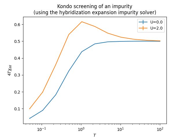
plt.title('Kondo screening of a magnetic impurity\n(CT-HYB hybridization-expansion solver)')
for un in range(len(Uvalues)):
    plt.errorbar(Tvalues, values[un], yerr=errors[un], label="U=%.1f"%Uvalues[un])
plt.xscale('log')
plt.legend()
plt.show()

The plot shows $4T\chi_{dd}$ versus temperature on a logarithmic scale. For $U = 0$ , the effective moment is approximately constant (non-interacting limit). For $U = 2$ , it decreases toward zero at low temperature, demonstrating the Kondo screening of the impurity spin by the conduction electrons.

Effective local moment vs temperature showing Kondo screening

Walkthrough Video

Classical Monte Carlo DMRG