DMRG-03 Ground State Energies

In this tutorial we put the dmrg code and the control parameters introduced in DMRG-01 to work on the simplest possible target: the ground state energy. We consider the spin-1/2 and spin-1 antiferromagnetic Heisenberg chains of length $L$ with open boundary conditions, introduced in DMRG-02:

Ground State Energies

When studying a model Hamiltonian, the first question we usually ask is what is the ground state $| \psi_0 \rangle$ and its energy $E_0$. For the Heisenberg chain of length $L$, and other similar systems, we might be more interested in the energy per site (or per bond) in the thermodynamic limit. Both of these will be considered below.

Fixed Length Ground State Energies

Consider chains of length $L=32,64,96,128$. Both for spin-1/2 and spin-1, set up ground state energy calculations for numbers of states $D=50,100,150,200,300$. For each length, tabulate the truncation error and the ground state energies as a function of $D$. Experiment carefully with the number of sweeps to assure that for a given length and number of states your result is actually converged.

1. For each system size and spin magnitude, try to establish the connection between the accuracy of the total energy and the truncation error by plotting total energy vs. truncation error.

2. Observe how the convergence in $D$ deteriorates with system size for spin-1/2 and spin-1, and compare the convergence behavior in the two cases, apart from a global factor of order of the length. Hint: What you should see is, that but for the global factor, the convergence for large system sizes is only weakly dependent of length for the spin-1 chain, but much more strongly dependent for the spin-1/2 chain. This is because the spin-1 chain physics is dominated by segments of length of the correlation length, whereas for the spin-1/2 chain there is no finite length scale because of criticality.

3. Try to extrapolate ground state energies for each chain length to the $D\rightarrow\infty$ limit.

The one dimensional S=1/2 Heisenberg chain

Single run

The first example consists of setting up a simulation for a spin-1/2 Heisenberg chain with 32 sites, and open boundary conditions, keeping 100 states.

Using parameter files

The parameter file spin_one_half sets the most important parameters:

LATTICE="open chain lattice"
MODEL="spin" 
CONSERVED_QUANTUMNUMBERS="N,Sz" 
Sz_total=0
J=1
SWEEPS=4
NUMBER_EIGENVALUES=1
L=32 
{MAXSTATES=100}

Using the following sequence of commands you can first convert the input parameters to XML and then run the application dmrg:

parameter2xml spin_one_half
dmrg --write-xml spin_one_half.in.xml

The output file spin_one_half.task1.out.xml contains all the computed quantities and can be viewed with a standard internet browser.

DMRG will perform four sweeps, (four half-sweps from left to right and four half-sweeps from right to left) growing the basis in steps of MAXSTATES/(2*SWEEPS) until reaching the MAXSTATES=100 value we have declared. This is a convenient default option, but the number of states can be customized, as we show in the spin S=1 example below.

Using Python

To set up and run the simulation in Python we use the script spin_one_half.py. The first part of this script imports the required modules, prepares the input files as a list of Python dictionaries, writes the input files and runs the application:

import pyalps
import numpy as np
import matplotlib.pyplot as plt
import pyalps.plot

parms = [ { 
        'LATTICE'                   : "open chain lattice", 
        'MODEL'                     : "spin",
        'CONSERVED_QUANTUMNUMBERS'  : 'N,Sz',
        'Sz_total'                  : 0,
        'J'                         : 1,
        'SWEEPS'                    : 4,
        'NUMBER_EIGENVALUES'        : 1,
        'L'                         : 32,
        'MAXSTATES'                 : 100
       } ]

input_file = pyalps.writeInputFiles('parm_spin_one_half',parms)
res = pyalps.runApplication('dmrg',input_file,writexml=True)

To run this, in your computer terminal type:

python spin_one_half.py

We now have the same output files as in the command line version.

Next, we load the properties of the ground state measured by the DMRG code:

data = pyalps.loadEigenstateMeasurements(pyalps.getResultFiles(prefix='parm_spin_one_half'))

and print them to the terminal:

for s in data[0]:
    print(s.props['observable'], ':', s.y[0])

Additionally, we can load detailed data for each iteration step:

iter = pyalps.loadMeasurements(pyalps.getResultFiles(prefix='parm_spin_one_half'),
                          what=['Iteration Energy','Iteration Truncation Error'])

The above allows us to look at how the DMRG algorithm converged to the final results.

We finally plot the convergence of various quantities as functions of iterations:

plt.figure()
pyalps.plot.plot(iter[0][0])
plt.title('Iteration history of ground state energy (S=1/2)')
plt.ylim(-15,0)
plt.ylabel('$E_0$')
plt.xlabel('iteration')

plt.figure()
pyalps.plot.plot(iter[0][1])
plt.title('Iteration history of truncation error (S=1/2)')
plt.yscale('log')
plt.ylabel('error')
plt.xlabel('iteration')

plt.show()

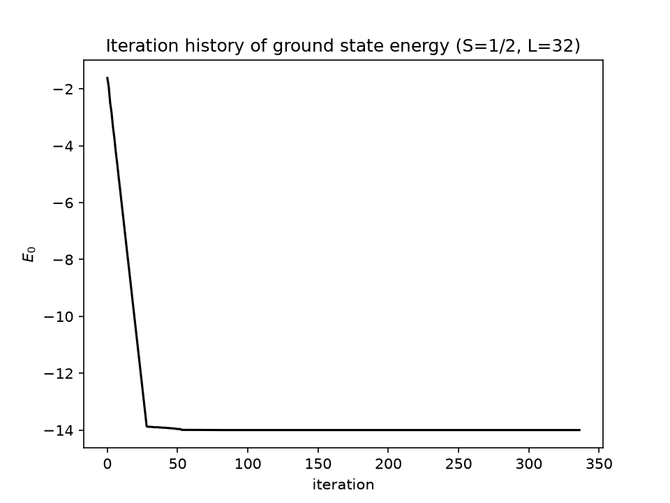
For the single run above (L=32, MAXSTATES=100, J=1), the ground state energy warms up during the infinite-system growth and settles to its converged value $E_0=-13.9973156\cdot J$ within about 50 iterations. Since the ground state energy is extensive, we divide by the 31 bonds to get the intensive per-bond energy $e_0/J = E_0/(31J)\approx-0.4515$, close to the exact thermodynamic-limit value $e_0/J=1/4-\ln2=-0.4431471806$ quoted in DMRG-02. The truncation error drops in a sawtooth pattern that bottoms out near machine precision ($\sim 10^{-16}$) at the end of each half-sweep and rises again as the next half-sweep begins:

Multiple runs

Using parameter files

We now proceed to illustrate how to setup several runs in a single parameter file spin_one_half_multiple. We shall use the example proposed in the tutorial, and simulate a chain of length L=32, changing the number of DMRG states (we shall use a smaller number of states for illustration purposes):

LATTICE="open chain lattice"
SWEEPS=4
CONSERVED_QUANTUMNUMBERS="N,Sz"
MODEL="spin", Sz_total=0
J=1
NUMBER_EIGENVALUES=1
L=32
{ MAXSTATES=20 }
{ MAXSTATES=40 }
{ MAXSTATES=60 }

As we can see, the main difference with the previous example exists in the parameters encoded in the brackets. As before, we run:

parameter2xml spin_one_half_multiple
dmrg --write-xml spin_one_half_multiple.in.xml

In this case, we will find three output files spin_one_half_multiple.task#.out.xml containing the results.

Using Python

The script spin_one_half_multiple.py sets up three Python dictionaries of parameters with differing MAXSTATES:

parms= []
for m in [20,40,60]:
    parms.append({ 
        'LATTICE'                   : "open chain lattice", 
        'MODEL'                     : "spin",
        'CONSERVED_QUANTUMNUMBERS'  : 'N,Sz',
        'Sz_total'                  : 0,
        'J'                         : 1,
        'SWEEPS'                    : 4,
        'NUMBER_EIGENVALUES'        : 1,
        'L'                         : 32,
        'MAXSTATES'                 : m
       })

After writing parameter files, running the dmrg application, and loading the results in the same way as for the single run above, we can print the measurements from all runs:

for run in data:
    for s in run:
        print(s.props['observable'], ':', s.y[0])

The one dimensional S=1 Heisenberg chain

The S=1 Heisenberg chain requires some special treatment due to the open boundary conditions. As explained in DMRG-01, we need to include two sites at both ends of the chain with a spin S=1/2 on each of them. This requires defining a new lattice file for the simulation. As it turns out, there is not a straightforward way to do this, so we will have to do it manually. To simplify the process, we have included a simple Python script build_lattice.py that will generate the lattice for us. The only input is the number of sites in the lattice.

Lattice

An open S=1 Heisenberg chain hosts a free effective spin-1/2 at each end (the origin of the fourfold ground-state degeneracy discussed in DMRG-04), which pollutes the low-energy spectrum used to extract bulk quantities. Capping the chain with an explicit spin-1/2 at each end absorbs these edge states, leaving a clean bulk spectrum to work with. This is exactly what build_lattice.py encodes: the same open chain as the S=1/2 case above, but with the two boundary sites given local_S0 instead of the bulk local_S1:

Regular open chain (5 sites, all spin S=1):

      J       J       J       J
  o-------o-------o-------o-------o
  1       2       3       4       5
  S=1     S=1     S=1     S=1     S=1


Open chain with the two special edges added for the S=1 tutorial (7 sites):

      J       J       J       J       J       J
  o-------o-------o-------o-------o-------o-------o
  0       1       2       3       4       5       6
  S=1/2   S=1     S=1     S=1     S=1     S=1     S=1/2

For instance, by typing:

python build_lattice.py 6

we shall obtain the output:

<LATTICES>
<GRAPH name = "open chain lattice with special edges" dimension="1" vertices="6" edges="5">
<VERTEX id="1" type="0"><COORDINATE>0</COORDINATE></VERTEX>
<VERTEX id="2" type="1"><COORDINATE>2</COORDINATE></VERTEX>
<VERTEX id="3" type="1"><COORDINATE>3</COORDINATE></VERTEX>
<VERTEX id="4" type="1"><COORDINATE>4</COORDINATE></VERTEX>
<VERTEX id="5" type="1"><COORDINATE>5</COORDINATE></VERTEX>
<VERTEX id="6" type="0"><COORDINATE>6</COORDINATE></VERTEX>
<EDGE source="1" target="2" id="1" type="0" vector="1"/>
<EDGE source="2" target="3" id="2" type="0" vector="1"/>
<EDGE source="3" target="4" id="3" type="0" vector="1"/>
<EDGE source="4" target="5" id="4" type="0" vector="1"/>
<EDGE source="5" target="6" id="5" type="0" vector="1"/>
</GRAPH>
</LATTICES>

As we can see, the lattice is defined as a one-dimensional graph that contains six vertices, and edges connecting nearest neighbors. The first and last vertices are of type “0”, while the others are of type “1”. We shall use this definition to implement the model on top of this lattice, which should contain information about the degrees of freedom living on these vertices.

The way to do this is by specifying the parameters:

local_S0=0.5
local_S1=1

To run a lattice with 32 sites we shall then type:

python build_lattice.py 32 > my_lattice.xml

Using parameter files

Let us see how the final parameter file spin_one should look like:

LATTICE_LIBRARY="my_lattice.xml"
LATTICE="open chain lattice with special edges"
MODEL="spin"
local_S0=0.5
local_S1=1
CONSERVED_QUANTUMNUMBERS="N,Sz"
Sz_total=0
J=1
SWEEPS=4
NUMBER_EIGENVALUES=1
{MAXSTATES=100}

Clearly, it is cumbersome to repeat this process for each system size. One way to simplify it even further is to write a script to do it for us automatically. A simpler approach is to define all the lattices we need in a lattice library. We have included a my_lattices.xml file with lattices of sizes $L=32,64,96,128,192$. All we have to do is modify the previous parameter file by replacing the lattice definition as follows:

LATTICE_LIBRARY="my_lattices.xml"
LATTICE="open chain lattice with special edges 32"

where we have included the lattice size in the name.

Using Python

The script spin_one.py defines the parameters in a Python dictionary:

parms = [ { 
        'LATTICE_LIBRARY'           : 'my_lattice.xml',
        'LATTICE'                   : 'open chain lattice with special edges',
        'MODEL'                     : 'spin',
        'local_S0'                  : '0.5',
        'local_S1'                  : '1',
        'CONSERVED_QUANTUMNUMBERS'  : 'N,Sz',
        'Sz_total'                  : 0,
        'J'                         : 1,
        'SWEEPS'                    : 4,
        'NUMBER_EIGENVALUES'        : 1,
        'MAXSTATES'                 : 100
       } ]

Apart from parameter and file name changes, it is the same as the spin_one_half.py script explained above.

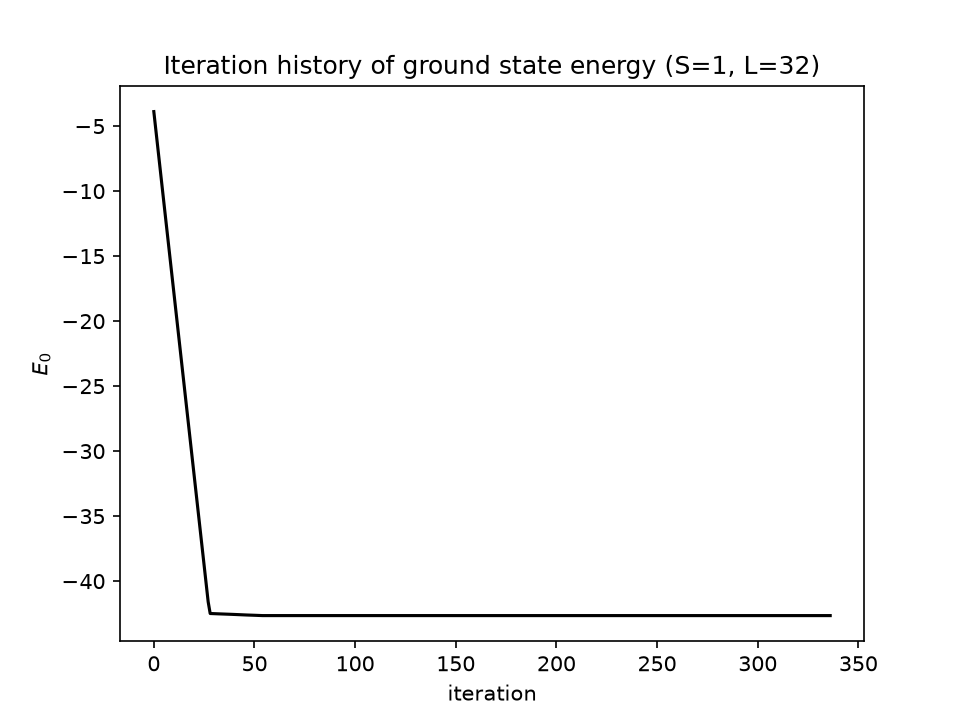
For this S=1 single run (L=32, MAXSTATES=100, J=1), the ground state energy warms up during the infinite-system growth and settles to its converged value $E_0=-42.6513851\cdot J$ within about 30 iterations. Dividing by the 31 bonds gives the intensive per-bond energy $e_0/J = E_0/(31J)\approx-1.3759$, close to the numerical thermodynamic-limit value $e_0/J=-1.401484039$ quoted in DMRG-02, as expected for a finite chain — even with the special edges added to suppress boundary effects. The truncation error shows the same sawtooth convergence pattern as the spin-1/2 case above, bottoming out near machine precision at the end of each half-sweep and rising again as the next half-sweep begins:

Multiple runs

Using parameter files

Same as for the spin S=1/2 case, we can now setup multiple runs in a single parameter file named spin_one_multiple as follows:

LATTICE_LIBRARY="my_lattices.xml"
LATTICE="open chain lattice with special edges 32"
MODEL="spin"
local_S0=0.5
local_S1=1
CONSERVED_QUANTUMNUMBERS="N,Sz"
Sz_total=0
J=1 
NUMBER_EIGENVALUES=1 
SWEEPS=4
{ MAXSTATES=20 } 
{ MAXSTATES=40 }
{ MAXSTATES=60 }

Using Python

The same runs can be set up with the script spin_one_multiple.py, which can be obtained from the corresponding spin-1/2 script by replacing the parameters.

Ground State Energies Per Site (Bond)

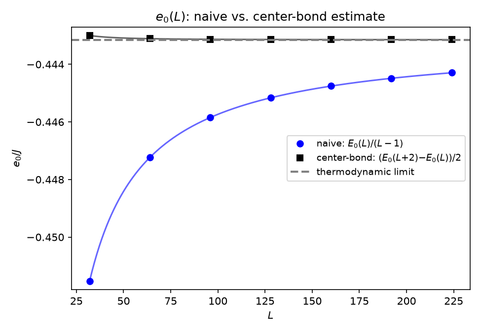
If we look closely at the Hamiltonian, the energy of a chain of length $L$ does not sit on the $L$ sites, but on the $L-1$ bonds. A first (naive) attempt therefore consists of taking the results of the last simulations and calculating:

The correct approach is to eliminate the effect of the open boundary conditions by considering the energy of one bond at the center of the chain. There are two ways of doing this.

1. Calculate the ground state energy of two chains of length $L$ and $L+2$, again for the lengths already mentioned above, and calculate $e_0/J = (E_0(L+2) - E_0 (L))/2$ as the energy per bond.

2. The less costly and usual way would be to use correlators (as discussed further in DMRG-06) between neighboring sites:

   $$e_0/J = \frac{1}{2} (\langle S^+_i S^-_{i+1}\rangle + \langle S^-_i S^+_{i+1}\rangle ) + \langle S^z_i S^z_{i+1} \rangle$$

for sites $i$ and $i+1$ at the chain center.

Summary

DMRG converges the ground-state energy of both the spin-1/2 and spin-1 open chains to high accuracy within a few dozen iterations, but the naive per-bond energy estimate $E_0(L)/(L-1)$ is a poor stand-in for the thermodynamic-limit energy per bond, since it does not correct for the open boundary conditions; a center-bond estimate is needed instead.

Questions

• Apart from a global factor set by the chain length, do you see a difference between how the convergence in $D$ deteriorates with system size for the spin-1/2 chain versus the spin-1 chain?
• Comparing $e_0/J=E_0(L)/(L-1)$ to the exact thermodynamic-limit energies per site quoted in DMRG-02, do you get values that are really close? What is wrong with the underlying assumption? (see hint)
• Using $e_0/J=(E_0(L+2)-E_0(L))/2$ instead, for the same chain lengths, what do the results look like now? (see hint)