DMRG-04 Gaps

Calculating The Gap

As already mentioned in DMRG-02, the energy gap of a quantum system is given by the energy difference between the first excited state and the ground state:

in the thermodynamic limit. This means we have to solve two problems, (i) the calculation of:

for finite system sizes and (ii) the extrapolation of $\Delta (L)$ to the thermodynamic limit $L= \infty$. The latter is not specific to DMRG, but because of DMRG’s preference for open boundary conditions it is somewhat more complicated than in the more usual case of periodic boundary conditions.

Getting The Gap For Finite Systems

Obviously, we have to be able to get access to the first excited state and its energy. DMRG fundamentally knows two ways of doing this, a pedestrian way which always works, but is not as neat, and a smarter way, which is very clean, but does not work under all circumstances.

1. The pedestrian way is to set up a DMRG calculation that calculates both states at the same time. However, for a given number of states the accuracy will somewhat decrease, as two different quantum states both have to be described accurately.

2. The smarter way reduces the gap calculation to the calculation of two ground states. In many quantum systems, the ground state and the first excited state differ by a good quantum number and therefore are both ground states in the respective sectors. For example, for the spin-1/2 chain, the ground state is a singlet of total spin 0, and hence the ground state in the sector of magnetization 0. The first excited state is a triplet of total spin 1, i.e. consists of one excited state of magnetization 0, and the ground states of the sectors of magnetization +1 and -1, respectively. It can, therefore, be calculated as the ground state in magnetization sector +1.

Let us start by doing these calculation for the spin-1/2 chain.

Example: without quantum numbers

Parameters and lattice

      J       J       J       J
  o-------o-------o-------o-------o
  1       2       3       4       5
  S=1/2   S=1/2   S=1/2   S=1/2   S=1/2

The built-in open chain lattice, spin-1/2 on every site; see the ALPS lattice library for its definition and the other lattices available.

Using parameter files

In this example below, we include a line in the parameter file for the spin S=1/2 chain spin_one_half_gap to tell the code that we also want to calculate the energy for the first excited state. The algorithm will build a density matrix targeting two states: the ground-state, and the first excited state, both in the same subspace with Sz=0. Since the first excited state is a triplet, this will yield the singlet-triplet gap:

LATTICE="open chain lattice"
MODEL="spin"
CONSERVED_QUANTUMNUMBERS="N,Sz"
Sz_total=0
J=1
SWEEPS=4
{L=32, MAXSTATES=100
NUMBER_EIGENVALUES=2}

Notice that we only added the last line, specifying the number of eigenstates to calculate. By targeting both states, the algorithm ensures that both are represented accurately. However, this is not quite true if we keep only 100 states. Compare the energy for the ground-state obtained with the present parameter file with the previous simulation targeting only the ground state.

It is important to notice that the entanglement entropy in this example is totally meaningless since the algorithm is calculating a density matrix mixing two states. In short, the algorithm targets both the ground state and first excited state in the $S_z=0$ sector, causing classical mixing uncertainty rather than pure quantum entanglement. To properly calculate entanglment entropy, one needs to independently diagonalize both the singlet and triplet sectors to avoid this mixing.

Using Python

The script spin_one_half_gap.py runs the same simulation as the spin-1/2 script from the DMRG-03 tutorial, except for changing the requested NUMBER_EIGENVALUES to two, and loads all data for these eigenstates:

import pyalps
import numpy as np
import matplotlib.pyplot as plt
import pyalps.plot

parms = [ { 
        'LATTICE'                   : "open chain lattice", 
        'MODEL'                     : "spin",
        'CONSERVED_QUANTUMNUMBERS'  : 'N,Sz',
        'Sz_total'                  : 0,
        'J'                         : 1,
        'SWEEPS'                    : 4,
        'L'                         : 32,
        'MAXSTATES'                 : 100,
        'NUMBER_EIGENVALUES'        : 2
       } ]

input_file = pyalps.writeInputFiles('parm_spin_one_half_gap',parms)
res = pyalps.runApplication('dmrg',input_file,writexml=True)

data = pyalps.loadEigenstateMeasurements(pyalps.getResultFiles(prefix='parm_spin_one_half_gap'))

While iterating over all measurements, we then extract the energies:

energies = np.empty(0)
for s in data[0]:
    if s.props['observable'] == 'Energy':
        energies = s.y
    else:
        print(s.props['observable'], ':', s.y[0])

and calculate the gap:

energies.sort()
print('Energies:', end=' ')
for e in energies:
    print(e, end=' ')
print('\nGap:', abs(energies[1]-energies[0]))

Example: with quantum numbers

Parameters and lattice

      J       J       J       J
  o-------o-------o-------o-------o
  1       2       3       4       5
  S=1/2   S=1/2   S=1/2   S=1/2   S=1/2

The built-in open chain lattice, spin-1/2 on every site; see the ALPS lattice library for its definition and the other lattices available.

To calculate the singlet-triplet gap taking advantage of quantum number conservation we need to perform two independent simulations, one with Sz=0, and another one with Sz=1. The difference of the two energies will yield the gap.

Using parameter files

This means that we only need to change the value of Sz_total in the spin_one_half parameter file:

LATTICE="open chain lattice"
MODEL="spin"
CONSERVED_QUANTUMNUMBERS="N,Sz"
Sz_total=1
SWEEPS=4
J=1
{L=32, MAXSTATES=40}

You can download this file from here: spin_one_half_triplet.

Using Python

The script spin_one_half_triplet.py runs a simulation for both Sz sectors defined by two Python dictionaries with the parameters:

import pyalps
import numpy as np
import matplotlib.pyplot as plt
import pyalps.plot

parms = []
for sz in [0,1]:
    parms.append( { 
        'LATTICE'                   : "open chain lattice", 
        'MODEL'                     : "spin",
        'CONSERVED_QUANTUMNUMBERS'  : 'N,Sz',
        'Sz_total'                  : sz,
        'J'                         : 1,
        'SWEEPS'                    : 4,
        'L'                         : 32,
        'MAXSTATES'                 : 40,
        'NUMBER_EIGENVALUES'        : 1
       } )
       
input_file = pyalps.writeInputFiles('parm_spin_one_half_triplet',parms)
res = pyalps.runApplication('dmrg',input_file,writexml=True)

After loading the results in the usual way, we print the measurements for both sectors and save the ground state energy for each Sz value in a dictionary:

data = pyalps.loadEigenstateMeasurements(pyalps.getResultFiles(prefix='parm_spin_one_half_triplet'))

# print results:
energies = {}
for run in data:
    print('S_z =', run[0].props['Sz_total'])
    for s in run:
        print('\t', s.props['observable'], ':', s.y[0])
        if s.props['observable'] == 'Energy':
            sz = s.props['Sz_total']
            energies[sz] = s.y[0]

Then, we can calculate the gap as the energy difference between the Sz=1 and Sz=0 sectors:

print('Gap:', energies[1]-energies[0])

Extrapolating The Gap To The Thermodynamic Limit

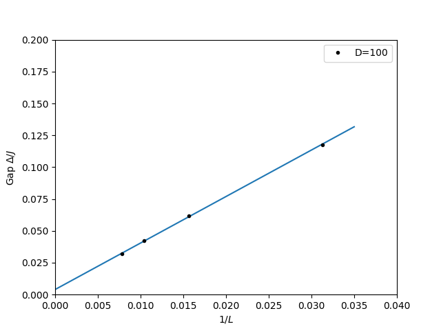
A first attempt fixes $D=50,100,150$ and takes the gap for lengths $L=32,64,96,128$, plotting the gap against $1/L$ at fixed $D$. For small $D$ the results do not lie on a straight line through 0 but curve up from it, and the behaviour improves as $D$ grows.

In a second, more meaningful attempt, fix the lengths $L=32,64,96,128$ and vary $D=50,100,150,200$ in order to extrapolate the gap for each fixed length in $D$ (or, as explained above, the truncation error), and plot the gap versus $1/L$ using these extrapolated values.

The plot below shows the spin-1/2 singlet-triplet gap versus $1/L$ at fixed $D=100$: the four points sit close to a straight line through a small but clearly nonzero intercept, illustrating exactly the frustration described below — with only these four chain lengths it is hard to tell a genuinely vanishing gap from a very small finite one.

Modify the file spin_one_half_multiple to setup all the runs for Sz=0 and Sz=1, for different system sizes and different number of states. Use five sweeps, and extrapolate the value of the gap following the procedure outlined in the tutorial.

The case of the spin-1/2 chain is a bit frustrating: even pushing the computer to its limits, the most that can be said is that the gap appears extremely small and therefore is likely to vanish. Nothing in the data rules out a gap of, say, $e^{-50}$. This is a sobering reminder of the limits of even a highly accurate numerical method.

We therefore turn to a more rewarding case, the gap of the spin-1 antiferromagnetic Heisenberg chain.

Here, there is a nasty twist, which we will only state and perform at the moment, but explain later: Calculate the gap not between the ground states of the magnetization sectors 0 and 1, but 1 and 2. If you wish, do it also for 0 and 1, for later reference, but the following refers to 1 and 2.

Assume you have $\Delta (L)$ within your machine’s precision, either by a suitable extrapolation as discussed above or by a very high accuracy calculation. If you don’t want to do the former, calculate the gap for system sizes $L=8,16,32,48,64,96,128,192,256$ all with $D=300$ states and 5 sweeps.

The effects of the open ends will decrease as $1/L$, so it makes sense to first plot the gaps $\Delta (L)$ versus $1/L$. This was already done in the spin-1/2 case to produce such a plot. What you see is a curve that is quite straight for small L and then starts bending upward. It would be ideal to have an idea of what the asymptotic behavior is (the curved part for long lengths), analytically or approximately, to extrapolate. It is common to produce a plot of the gap $\Delta (L)$ versus $1/L^2$ to do so.

The plot below shows the spin-1 gap versus $1/L^2$ at fixed $D=200$: the points now lie on a good straight line, extrapolating to an intercept close to the accepted Haldane gap $\Delta/J=0.41052$ (see DMRG-02) — a much better behaved extrapolation than the spin-1/2 case above, consistent with the $1/L^2$ convergence derived below.

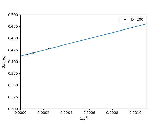
This procedure was in fact motivated by the following argument: from Haldane’s analysis of the spin-1 chain by the nonlinear sigma model, one expects that the lowest lying excitations (which for periodic boundary conditions can be labeled by a momentum $k$) are around $k=\pi$ and have an energy:

For the open boundary conditions, we may approximate $k-\pi$ by $1/L$ (think about a particle in a box), which gives a finite-system size gap of:

and indicates that in the asymptotic limit the convergence should essentially be as $1/L^2$.

For those that also did the gap between the ground states of magnetization sectors 0 and 1, show that the gap you get there is essentially zero. All others, take this result for granted. In fact, there is a very good reason why the spin-1 chain shows this peculiar behavior for open boundary conditions that can be found analytically, but even if we were not so fortunate as to know it, we could detect the problem right away! This can be done by the observation of local observables.

Summary

DMRG resolves the (likely vanishing) gap of the critical spin-1/2 chain and the finite Haldane gap of the spin-1 chain, but the two require different extrapolation strategies — $1/L$ for the near-gapless case versus $1/L^2$ for the gapped one — reflecting their different long-distance physics; DMRG-05 explains why the spin-1 gap must specifically be taken between magnetization sectors 1 and 2.

Questions

• Why does the curvature of the gap-vs-$1/L$ plot straighten out as $D$ is increased at fixed chain lengths?
• Extrapolating the gap in $D$ (or in the truncation error) at each fixed length before plotting versus $1/L$: what does the plot look like now, compared to the first attempt at fixed $D$?
• If you extrapolate only the linear (small-$L$) part of the $\Delta(L)$ vs. $1/L$ curve for the spin-1 chain naively, what gap do you obtain, and is it over- or underestimated? (This is relevant for situations where the correlation length of the chain is so long that it becomes hard to see the asymptotic behavior on reachable length scales.)
• What gap do you read off if you instead take the longest chain you have, and is it over- or underestimated?
• Plotting the gap as $\Delta(L)$ versus $1/L^2$ instead of $1/L$: what does the curve now look like for large lengths, and what gap do you extrapolate?
• How close does your extrapolated gap come to the accepted value $\Delta/J=0.41052$ from DMRG-02?
• The gap between magnetization sectors 0 and 1 is essentially zero, while the gap between sectors 1 and 2 is finite. Why is the finite gap the physically correct one and the vanishing gap the wrong one — is this a physics lottery?