DMRG-05 Local Observables
Excitations
Observables linked to one specific site are known as local observables. In the case of spin chains, the meaningful local observable is the local magnetization . Its spatial profile tells us where the magnetization sits, which lets each magnetization sector be associated with a particular energy mode: a boundary mode costing almost nothing, or a bulk magnon costing the Haldane gap. We use the spatial profiles of the magnetizations below to analyze the spin-1 chain subject to two different boundary conditions.
Spin-1 boundary: the uniform chain
Lattice and excitations
      J       J       J       J
  o-------o-------o-------o-------o
  1       2       3       4       5
  S=1     S=1     S=1     S=1     S=1
We begin with the uniform chain, in which every site — including the two ends — carries spin 1. The calculation below uses a chain of spin-1 sites with states, taking the local magnetization of the ground state in each of the magnetization sectors 0, 1 and 2, plotted against the site index .
Sector 0 gives a curve which is large at both chain ends but equal and opposite there, so that it sums to zero. Sector 1 also has a magnetization which is again concentrated at the chain ends, but now with the same sign at both. Finally, sector 2 possesses a magnetization which is both at the chain ends and in the bulk of the chain, this being the sector we will be most interested in. Note that the boundary modes exist only because the chain has open ends: they would be absent on a ring. Open boundaries are the natural geometry for DMRG, which makes it an ideal tool to study edge modes. As we will see, these magnetizations describe the character of the first and second excitations.
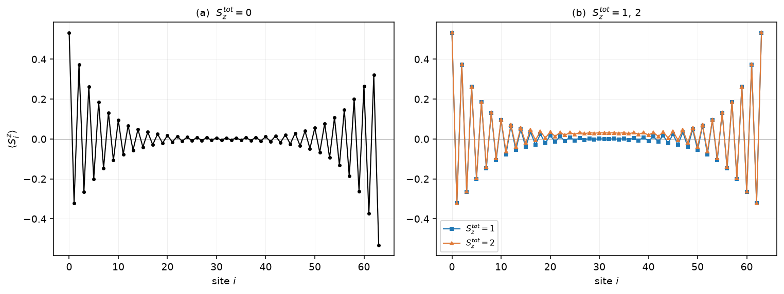
Figure 1. Uniform spin-1 chain, , . (a) : the two edge spins point opposite ways, so the profile is large at both ends but sums to zero. (b) and : the ends carry the same weight in both, and only sector 2 adds magnetization in the bulk.
Sectors 0 and 1 are in fact degenerate: the state carrying costs essentially no energy, since it only reorients the boundary. The first bulk excitation therefore has to be extracted by comparing sectors 1 and 2, for the reason set out just below. The moral of the story is that by looking at this local observable, we can distinguish boundary from bulk excitations in the spin-1 chain.
Which states the sectors contain
The reason sectors 0 and 1 are degenerate is that they hold the same kind of state. An open spin-1 chain in the Haldane phase carries an emergent spin-1/2 at each end: in the valence-bond picture every spin-1 is two spin-1/2s paired with its neighbors, and at an open end one half is left without a partner. Two such spin-1/2s combine into four nearly degenerate states, which is often transcribed as a tensor product in terms of a direct sum:
This expression says combining two spin-1/2s results in one singlet and one triplet, split only by an effective coupling transmitted through the gapped bulk. This decays as with sites, so at that splitting is already below .
Reading the magnetization sectors against that multiplet:
| state | the two emergent edge spins | |
|---|---|---|
| 0 | singlet () or triplet member (), degenerate here | / for either; / for a superposition of them |
| 1 | triplet member — both edge spins up | / |
| 2 | edge triplet plus one bulk magnon | / , with weight added in the bulk |
The above is the total carried by each emergent edge spin, not the value on the end site itself. That spin is spread over roughly sites with alternating sign, so the site-resolved magnetization at the very end of the chain comes out near in Figure 1, decaying into the bulk.
Two edge spin-1/2s can supply at most between them. Sector 2 is therefore the first sector that cannot be built from the boundary alone and is forced to contain a magnon, which is exactly why the bulk gap is the difference between sectors 1 and 2: the edge contribution is identical on both sides and cancels,
Parameters
| Parameter | Meaning | Value |
|---|---|---|
LATTICE | built-in open chain, no lattice file needed (see the ALPS lattice library) | open chain lattice |
L | number of sites, all spin-1 | 64 |
local_S | spin quantum number on every site | 1 |
MODEL | quantum spin model | spin |
CONSERVED_QUANTUMNUMBERS | quantum numbers held fixed | N,Sz |
Sz_total | magnetization sector targeted | 0, 1, 2 (one run each) |
J | nearest-neighbor Heisenberg coupling | 1 |
SWEEPS | number of DMRG finite-size sweeps | 6 |
NUMBER_EIGENVALUES | eigenstates requested per sector | 1 |
MAXSTATES | bond dimension kept after truncation | 100 |
MEASURE_LOCAL[...] | site-resolved observable to record | Sz |
Running it
The uniform chain needs no lattice file — open chain lattice with local_S=1 is enough. The parameter file spin_one_uniform sets up three runs, one per sector:
LATTICE="open chain lattice"
MODEL="spin"
local_S=1
CONSERVED_QUANTUMNUMBERS="N,Sz"
J=1
L=64
NUMBER_EIGENVALUES=1
SWEEPS=6
MAXSTATES=100
MEASURE_LOCAL[Local magnetization]=Sz
{ Sz_total=0 }
{ Sz_total=1 }
{ Sz_total=2 }

parameter2xml spin_one_uniform
dmrg --write-xml spin_one_uniform.in.xml
or equivalently from Python, with spin_one_uniform.py:
import pyalps
parms = []
for sz in [0,1,2]:
    parms.append( {
        'LATTICE'                   : 'open chain lattice',
        'MODEL'                     : 'spin',
        'local_S'                   : '1',
        'CONSERVED_QUANTUMNUMBERS'  : 'N,Sz',
        'Sz_total'                  : sz,
        'J'                         : 1,
        'L'                         : 64,
        'SWEEPS'                    : 6,
        'NUMBER_EIGENVALUES'        : 1,
        'MAXSTATES'                 : 100,
        'MEASURE_LOCAL[Local magnetization]' : 'Sz'
    } )
input_file = pyalps.writeInputFiles('parm_spin_one_uniform',parms)
pyalps.runApplication('dmrg',input_file,writexml=True)
Loading the results and plotting against the site index reproduces Figure 1:
import numpy as np, matplotlib.pyplot as plt
data = pyalps.loadEigenstateMeasurements(
    pyalps.getResultFiles(prefix='parm_spin_one_uniform'))
for run in data:
    for s in run:
        if s.props['observable'] == 'Local magnetization':
            y = np.real(np.asarray(s.y).flatten())
            plt.plot(np.arange(len(y)), y, marker='o', ms=3,
                     label='$S_z^{tot} = %g$' % float(s.props['Sz_total']))
plt.xlabel('site $i$'); plt.ylabel(r'$\langle S^z_i \rangle$')
plt.legend(); plt.show()
A useful check on any of these runs is that equals exactly; if it does not, the run is not converged.
Spin-1/2 boundary: absorbing the edge states
Lattice and excitations
      J       J       J       J       J       J
  o-------o-------o-------o-------o-------o-------o
  0       1       2       3       4       5       6
  S=1/2   S=1     S=1     S=1     S=1     S=1     S=1/2
Now we keep the same spin-1 sites and attach an extra spin-1/2 at each end, coupled to the chain by the same . The degeneracy found above is a property of the ends, not of the bulk, so it can be removed without touching the phase: the attached spin-1/2 gives the dangling emergent spin-1/2 a partner to form a singlet with, screening it much as a Kondo impurity is screened. Two half-integer spins combine into an integer representation, which can be gapped symmetrically, so the fourfold manifold collapses to a single ground state. A spin-1 cap would not do this — it would simply lengthen the chain and reproduce the same free edge state one site further in.
Repeat the calculation on this lattice, again for sectors 0, 1 and 2. The excitations now behave quite differently:
- Sector 0 is a unique singlet, and vanishes on every site — there is no edge degree of freedom left to orient.
- Sector 1 no longer costs nothing. With the boundary states absorbed, the cheapest way to add one unit of is a bulk magnon, and the magnetization appears spread through the interior rather than pinned at the ends.
- Sector 2 is two magnons, and the profile develops the corresponding structure in the bulk.
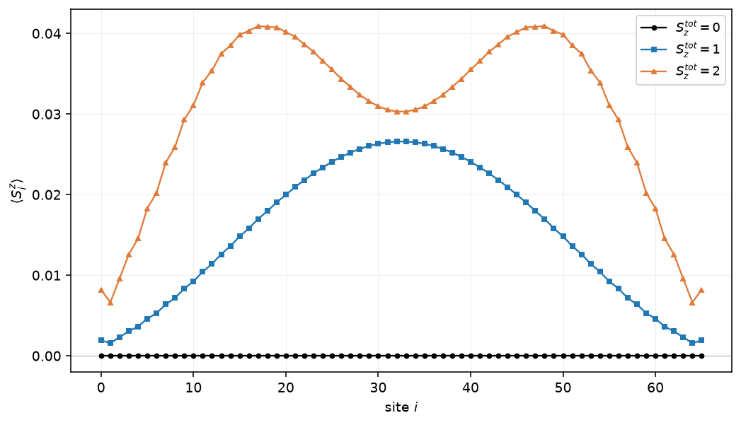
Figure 2. Spin-1 chain with a spin-1/2 attached at each end, , all three sectors on one axis. Note the vertical scale: the profiles are more than an order of magnitude smaller than in Figure 1, and the ends are now the quietest part of the chain rather than the loudest.
Nothing about the bulk has changed: the Haldane gap, the correlation length and the string order are properties of the interior, and cutting the capped chain anywhere in the middle would expose free emergent spin-1/2s at the new ends again. What changes is only which sector first requires a bulk excitation. With spin-1 ends the gap must be read between sectors 1 and 2; with spin-1/2 ends the boundary states are gone and the same gap appears between sectors 0 and 1.
Parameters
| Parameter | Meaning | Value |
|---|---|---|
LATTICE_LIBRARY | custom lattice written by build_lattice.py | my_lattice.xml |
LATTICE | open chain whose end vertices carry a separate type | open chain lattice with special edges |
| — | total sites: 64 spin-1 plus one spin-1/2 at each end | 66 |
local_S0 | spin on the two end sites | 0.5 |
local_S1 | spin on the 64 interior sites | 1 |
MODEL | quantum spin model | spin |
CONSERVED_QUANTUMNUMBERS | quantum numbers held fixed | N,Sz |
Sz_total | magnetization sector targeted | 0, 1, 2 (one run each) |
J | nearest-neighbor Heisenberg coupling | 1 |
SWEEPS | number of DMRG finite-size sweeps | 6 |
NUMBER_EIGENVALUES | eigenstates requested per sector | 1 |
MAXSTATES | bond dimension kept after truncation | 100 |
MEASURE_LOCAL[...] | site-resolved observable to record | Sz |
Running it
The capped chain does need a lattice file. build_lattice.py writes an open
chain whose two end vertices are given a separate type, so they can be assigned
a different spin; pass it the total number of sites, i.e. two more than the
number of spin-1 sites you want:
python build_lattice.py 66 > my_lattice.xmlThat gives 64 spin-1 sites with a spin-1/2 attached at each end. The parameter
file spin_one_capped is then the same as before apart from the lattice and the two local spins:
LATTICE_LIBRARY="my_lattice.xml"
LATTICE="open chain lattice with special edges"
MODEL="spin"
local_S0=0.5
local_S1=1
CONSERVED_QUANTUMNUMBERS="N,Sz"
J=1
NUMBER_EIGENVALUES=1
SWEEPS=6
MAXSTATES=100
MEASURE_LOCAL[Local magnetization]=Sz
{ Sz_total=0 }
{ Sz_total=1 }
{ Sz_total=2 }

parameter2xml spin_one_capped
dmrg --write-xml spin_one_capped.in.xml
or from Python, with spin_one_capped.py:
import pyalps
parms = []
for sz in [0,1,2]:
    parms.append( {
        'LATTICE_LIBRARY'           : 'my_lattice.xml',
        'LATTICE'                   : 'open chain lattice with special edges',
        'MODEL'                     : 'spin',
        'local_S0'                  : '0.5',
        'local_S1'                  : '1',
        'CONSERVED_QUANTUMNUMBERS'  : 'N,Sz',
        'Sz_total'                  : sz,
        'J'                         : 1,
        'SWEEPS'                    : 6,
        'NUMBER_EIGENVALUES'        : 1,
        'MAXSTATES'                 : 100,
        'MEASURE_LOCAL[Local magnetization]' : 'Sz'
    } )
input_file = pyalps.writeInputFiles('parm_spin_one_capped',parms)
pyalps.runApplication('dmrg',input_file,writexml=True)
Reading the results back works exactly as for the uniform chain, and gives Figure 2.
Magnetization in the spin-1/2 chain
Lattice
      J       J       J       J
  o-------o-------o-------o-------o
  1       2       3       4       5
  S=1/2   S=1/2   S=1/2   S=1/2   S=1/2
The same open chain, now with spin-1/2 on every site. There is no Haldane gap and no emergent boundary spin here, so none of the edge physics above applies.
Repeat a similar calculation for the spin-1/2 chain in the lowest magnetization sectors.
Parameters
| Parameter | Meaning | Value |
|---|---|---|
LATTICE | built-in open chain (see the ALPS lattice library) | open chain lattice |
L | number of sites | 64 |
MODEL | quantum spin model (default ) | spin |
CONSERVED_QUANTUMNUMBERS | quantum numbers held fixed | N,Sz |
Sz_total | magnetization sector targeted | 0, 1, 2 (one run each) |
J | nearest-neighbor Heisenberg coupling | 1 |
SWEEPS | number of DMRG finite-size sweeps | 6 |
NUMBER_EIGENVALUES | eigenstates requested per sector | 1 |
MAXSTATES | bond dimension | 100 |
MEASURE_LOCAL[...] | site-resolved observable | Sz |
Using parameter files
The following parameter file spin_one_half will accomplish this task:
LATTICE="open chain lattice"
MODEL="spin"
CONSERVED_QUANTUMNUMBERS="N,Sz"
SWEEPS=6
J=1
NUMBER_EIGENVALUES=1
MEASURE_LOCAL[Local magnetization]=Sz
L=64
MAXSTATES=100
{ Sz_total=0 }
{ Sz_total=1 }
{ Sz_total=2 }

parameter2xml spin_one_half
dmrg --write-xml spin_one_half.in.xml
Using Python
Apart from the obvious parameter changes, the script spin_one_half.py is the same as the spin_one_uniform script explained above.
Summary
The local magnetization profile cleanly separates boundary excitations from bulk excitations in the open spin-1 chain, which is why the physically relevant (bulk) gap studied in DMRG-04 must be read off between magnetization sectors 1 and 2 rather than 0 and 1.
Questions
- Repeating the local-magnetization calculation for the spin-1/2 chain in its lowest magnetization sectors, what do you observe, compared to the spin-1 case above?