DMRG-06 Correlations

Correlation Functions

The most important correlation functions in many-body physics are two-point correlators, i.e. correlators that involve two sites $i$ and $j$, such as $\langle S^+_i S^-_j \rangle$. Short-ranged ones determine energies (in the typical short-ranged Hamiltonians of correlation physics), long-ranged ones determine correlation lengths.

Another Go At The Energy Per Bond

As already mentioned in DMRG-02, the ground state energy per bond in both spin-1/2 and spin-1 chains are given by:

This gives the energy of each bond individually, but we are interested in the thermodynamic limit, where all bonds are on equal footing and hence should have the same energy unless there is some physical breaking of translational invariance. The bonds closest to this asymptotic behavior are those in the chain center, so the direct approach is to calculate $e_0(L/2)$ and extrapolate it first in $D$ for fixed $L$, then in $L$ at fixed $D$. It is worth inspecting $e_0(i)$ against $i$ first, for a few values of $D$ and $L$ that are not too small; the three contributions can also be examined individually before summing them, as a check of the program.

For the spin-1/2 chain, bond energies oscillate strongly between odd and even numbered bonds. This is because the open ends are felt very strongly, due to criticality, and because the spin-1/2 chain is on the verge of dimerization, i.e. a spontaneous breaking of translational symmetry of the ground state down to a periodicity of 2. It is therefore more meaningful to extrapolate the average energy of a strong and a weak bond, which gains a great deal of accuracy. This is a further demonstration of the value of inspecting the actual output of DMRG through local, or here almost local, observables.

Spin-Spin Correlations: Spin-1/2

Lattice and correlations

      J       J       J       J
  o-------o-------o-------o-------o
  1       2       3       4       5
  S=1/2   S=1/2   S=1/2   S=1/2   S=1/2

The plain open chain, spin-1/2 on every site.

For a relatively long chain, say $L=192$, the correlator $\langle S^z_i S^z_j \rangle$ is calculated for a range of increasing $D$.

The quantity plotted is $C_l = \langle S^z_{L/2-l/2} S^z_{L/2+l/2} \rangle$, with the positions rounded so that their separation is $l$. Centering the correlators on the chain makes boundary effects as small as possible; averaging over several correlators at the same separation is an equally valid alternative. Since a power law with critical exponent $\eta=1$ is expected (see DMRG-02), a log-log plot is appropriate, taking absolute values or dividing out the antiferromagnetic factor $(-1)^l$.

The result is a power law at short distances, crossing over to a faster, in fact exponential, decay at larger ones. This has two reasons: (i) the finite system size cuts off the power-law correlations; but as we took a large system size here, this should not matter too much. (ii) DMRG’s algorithmic structure effectively generates correlators which are superpositions of up to $D^2$ purely exponential decays, and therefore can only mimic power-laws by such superpositions - at large distances, the slowest exponential decay will survive all the others, replacing the power-law by an exponential law. Larger $D$ pushes this crossover further out.

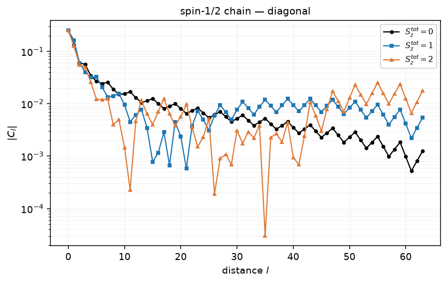
Figure 1. $|C_l|$ against separation $l$ for the spin-1/2 chain, $L=64$, $D=100$, in the three lowest magnetization sectors. The decay is far slower than in the spin-1 case below, as expected for a critical chain.

Parameters

Using parameter files

The following parameter file spin_one_half will setup this run for us (once again, for illustration we shall use a smaller system and number of states than the more realistic numbers stated above). The example uses a chain of length $L=64$ at $D=100$, with one run in each of the three lowest magnetization sectors, and 6 sweeps. The correlations should come out symmetric:

LATTICE="open chain lattice"
MODEL="spin"
CONSERVED_QUANTUMNUMBERS="N,Sz"
SWEEPS=6
J=1
NUMBER_EIGENVALUES=1
MEASURE_AVERAGE[Magnetization]=Sz
MEASURE_AVERAGE[Exchange]=exchange
MEASURE_LOCAL[Local magnetization]=Sz
MEASURE_CORRELATIONS[Diagonal spin correlations]=Sz
MEASURE_CORRELATIONS[Offdiagonal spin correlations]="Splus:Sminus"
L=64
MAXSTATES=100
{ Sz_total=0 }
{ Sz_total=1 }
{ Sz_total=2 }

parameter2xml spin_one_half
dmrg --write-xml spin_one_half.in.xml

Using Python

The script spin_one_half.py sets up one run per magnetization sector and loads the results:

import pyalps
import numpy as np
import matplotlib.pyplot as plt
import pyalps.plot
parms = []
for sz in [0,1,2]:
    parms.append( { 
        'LATTICE'                               : 'open chain lattice', 
        'MODEL'                                 : 'spin',
        'CONSERVED_QUANTUMNUMBERS'              : 'N,Sz',
        'Sz_total'                              : sz,
        'J'                                     : 1,
        'SWEEPS'                                : 6,
        'NUMBER_EIGENVALUES'                    : 1,
        'L'                                     : 64,
        'MAXSTATES'                             : 100,
        'MEASURE_AVERAGE[Magnetization]'        : 'Sz',
        'MEASURE_AVERAGE[Exchange]'             : 'exchange',
        'MEASURE_LOCAL[Local magnetization]'    : 'Sz',
        'MEASURE_CORRELATIONS[Diagonal spin correlations]'      : 'Sz',
        'MEASURE_CORRELATIONS[Offdiagonal spin correlations]'   : 'Splus:Sminus'
        } )
        
input_file = pyalps.writeInputFiles('parm_spin_one_half',parms)
res = pyalps.runApplication('dmrg',input_file,writexml=True)

data = pyalps.loadEigenstateMeasurements(pyalps.getResultFiles(prefix='parm_spin_one_half'))

Now we can extract e.g. $\langle S^z_iS^z_j\rangle$ correlations:

curves = []
for run in data:
    for s in run:
        if s.props['observable'] == 'Diagonal spin correlations':
            d = pyalps.DataSet()
            d.props['observable'] = 'Sz correlations'
            d.props['label'] = '$S_z^{tot}$ = '+str(s.props['Sz_total'])
            L = int(s.props['L'])
            d.x = np.arange(L)
       
            # sites with increasing distance l symmetric to the chain center
            site1 = np.array([int(-(l+1)/2.0) for l in range(0,L)]) + L/2
            site2 = np.array([int(  l   /2.0) for l in range(0,L)]) + L/2
            indices = L*site1 + site2
            d.y = abs(s.y[0][indices])
       
            curves.append(d)

and plot them vs. site distance:

plt.figure()
pyalps.plot.plot(curves)
plt.xscale('log')
plt.yscale('log')
plt.legend()
plt.title('Spin correlations in antiferromagnetic Heisenberg chain (S=1/2)')
plt.ylabel('correlations $| \\langle S^z_{L/2-l/2} S^z_{L/2+l/2} \\rangle |$')
plt.xlabel('distance $l$')
plt.show()

Spin-Spin Correlations: Spin-1

Lattice and correlations

      J       J       J       J       J       J
  o-------o-------o-------o-------o-------o-------o
  0       1       2       3       4       5       6
  S=1/2   S=1     S=1     S=1     S=1     S=1     S=1/2

Note this is the capped chain, with a spin-1/2 on each end site, not the uniform spin-1 chain. The caps absorb the emergent boundary spins (see DMRG-05), which keeps the correlators free of the edge-edge contribution that would otherwise dominate at large separation.

In the spin-1 chain, we do expect exponential decay (with an analytic modification), so the exponential nature of the correlators of DMRG should fit well. Again a long chain is used, say $L=192$, with $\langle S^z_i S^z_j \rangle$ calculated for increasing $D$.

The same $C_l = \langle S^z_{L/2-l/2} S^z_{L/2+l/2} \rangle$ is plotted, with positions rounded to separation $l$ as before. Since an exponential law is expected, a log-lin plot is used, again with the signs removed.

A correlation length extracted from the log-lin plot can be compared with the benchmark value $\xi=6.02$ quoted in DMRG-02. It depends on $D$, and in fact increases monotonically with it.

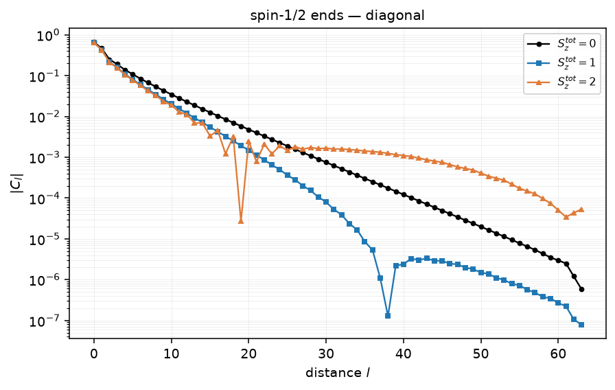
Figure 2. $|C_l|$ against separation $l$ for the capped spin-1 chain, $L=64$, $D=100$. The decay is exponential, and $\xi$ is read from the slope on this log-lin scale. On the uniform chain the same curve turns upward beyond $l \approx 30$, because at large separation both sites lie in the edge region and the correlator measures the boundary spins rather than the bulk — which is why the capped lattice is used here.

In fact, the calculation of correlation lengths is much harder to converge than that of the local quantities. This is due to the fact that a more profound algorithmic analysis reveals DMRG to be an algorithm geared especially well to the optimal representation of local quantities, not so much non-local ones as long-ranged correlators.

Parameters

Using parameter files

The parameter file spin_one looks much like the one for the previous example, but replacing the lattice and the model as follows. As above, the run shown here uses a smaller system than the more realistic $L=192$ quoted earlier: the 64-site capped chain from the lattice library, at $D=100$.

LATTICE_LIBRARY="my_lattices.xml"
LATTICE="open chain lattice with special edges 64"
MODEL="spin"
local_S0=0.5
local_S1=1
CONSERVED_QUANTUMNUMBERS="N,Sz"
Sz_total=0
SWEEPS=6
J=1
NUMBER_EIGENVALUES=1
MEASURE_AVERAGE[Magnetization]=Sz
MEASURE_AVERAGE[Exchange]=exchange
MEASURE_LOCAL[Local magnetization]=Sz
MEASURE_CORRELATIONS[Diagonal spin correlations]=Sz
MEASURE_CORRELATIONS[Offdiagonal spin correlations]="Splus:Sminus"
MAXSTATES=100

parameter2xml spin_one
dmrg --write-xml spin_one.in.xml

Using Python

The main difference of the script spin_one.py with respect to the previous one is the definition of lattice and model:

parms = []
L = 64
parms.append( { 
        'LATTICE_LIBRARY'                       : 'my_lattices.xml',
        'LATTICE'                               : 'open chain lattice with special edges '+str(L),
        'MODEL'                                 : 'spin',
        'local_S0'                              : 0.5,
        'local_S1'                              : 1,
        'CONSERVED_QUANTUMNUMBERS'              : 'N,Sz',
        'Sz_total'                              : 0,
        'J'                                     : 1,
        'SWEEPS'                                : 6,
        'NUMBER_EIGENVALUES'                    : 1,
        'MAXSTATES'                             : 100,
        'MEASURE_AVERAGE[Magnetization]'        : 'Sz',
        'MEASURE_AVERAGE[Exchange]'             : 'exchange',
        'MEASURE_LOCAL[Local magnetization]'    : 'Sz',
        'MEASURE_CORRELATIONS[Diagonal spin correlations]'      : 'Sz',
        'MEASURE_CORRELATIONS[Offdiagonal spin correlations]'   : 'Splus:Sminus'
    } )

After running the simulation, correlations can be extracted and plotted in the same way as before.

Sometimes There Is A Way Out

In the special case of the spin-1 chain, we have a loophole for the calculation of the correlation length, which is related to the weird observation that the first excitation was not a bulk excitation. It can be shown that a good toy model for a spin-1 chain is given as follows: at each site of a spin-1, you put two spin-1/2, and construct the spin-1 states from the triplet states of the two spin-1/2 at each site. The ground state is then approximated quite well by a state where you link two spin-1/2 on neighboring sites by a singlet state.

In this construction, for open boundary conditions (but not periodic ones), on the first and on the last site there will be two lonely spin-1/2 without partner. These two spin-1/2 particles can form 4 states among themselves, which in the toy model the ground state is four-fold degenerate. In the real spin-1 chain, this four-fold degeneracy (from one state of total spin 0 and three of total spin 1) is only achieved in the thermodynamic limit when the two spins are totally removed from each other. This is why there was no gap between magnetization sectors 0 and 1. The first bulk excitation needs magnetization 2.

To cure this, we can attach one spin-1/2 operator on each side of the lattice, taking the same bond Hamiltonian for these new sites, linking the two lonely spins by a singlet state. A gap then appears between magnetization sectors 0 and 1.

In order to calculate the correlation length, one can also play the following trick: attach only one spin-1/2 at one end. This means that the ground state will now be doubly degenerate, in magnetization sectors +1/2 or -1/2. We can characterize this by the boundary site where there is NO spin-1/2 attached carrying finite magnetization, that decays into the bulk, with the correlation length.

Summary

Correlation functions directly expose the qualitative difference between the two chains — power-law decay for the critical spin-1/2 chain versus exponential decay for the gapped spin-1 chain — while also showing where DMRG itself is least accurate, since long-ranged correlations converge far more slowly in $D$ than local quantities like the energy.

Questions

• Plotting $e_0(i)$ versus $i$ for various $D$ (not too small $L$): what do you observe for the spin-1 chain, and what for the spin-1/2 chain? Considering the three contributions to $e_0(i)$ individually before summing them, what relationship between them should exist?
• Has the correlation length converged by the time you reach $D=300$, and how does this compare to the convergence of local or quasi-local observables such as the magnetization or energy at the same $D$?
• For a chain of length $L=192$ and $D=200$, extracting the correlation length from the ground-state magnetization profile this way: what correlation length do you get, and how does it compare to $\xi=6.02$ from DMRG-02?