DMRG-08 Ground State Energies
In this tutorial we put the machinery developed in the DMRG-07 Introduction to work and compute ground state energies of the one-dimensional spinless-fermion chain with the ALPS dmrg application, following the same workflow as DMRG-03 for the spin chains.
Phenomena of interest
The spinless-fermion chain with nearest-neighbor repulsion — the – model — is the simplest interacting fermion model there is. It nevertheless contains the essential physics of one-dimensional metals: at weak coupling it is a Luttinger liquid, a critical metallic state with no quasiparticles, and at strong repulsion ( at half filling) it undergoes a transition into a gapped, charge-ordered insulator. Through the Jordan–Wigner transformation derived in the Introduction, it is exactly the XXZ spin chain in disguise, so every result obtained here can be cross-checked against the spin-chain tutorials. As in DMRG-03, we start with the most basic observable — the ground state energy — computed at two points of the phase diagram where exact reference values exist: the free-fermion point , and the interaction strength that maps onto the isotropic Heisenberg chain of DMRG-03.
The model
We study the – Hamiltonian on an open chain of sites,
with hopping amplitude , nearest-neighbor repulsion , and a (possibly site-dependent) chemical potential . The model is integrable: via the Jordan–Wigner transformation it is equivalent to the XXZ chain solved exactly by Yang and Yang, and its critical phase is the standard lattice realization of the Luttinger liquid.
The dictionary from the Introduction, applied to an open chain bond by bond, reads:
where is the coordination number of site ( in the bulk, at the two ends). The XXZ chain therefore equals the – model with the site-dependent chemical potential , up to the constant — a bookkeeping detail that we will exploit below to benchmark against DMRG-03.
Running fermions in the boson basis
hardcore boson with exactly the same parameters (t, V, mu#) and the same conserved quantum number N as spinless fermions, so every parameter file below sets MODEL="hardcore boson". This is not just a convenience: the classic dmrg application does not treat the fermionic sign bookkeeping of MODEL="spinless fermions" reliably. DMRG-10 makes the case in full, with the energies and convergence of the two models side by side.Choice of method
At half filling the relevant Hilbert-space sector has dimension:
far beyond the reach of full or sparse diagonalization. DMRG is the method of choice for one-dimensional ground states: each of the runs below (a 32-site chain with up to kept states and 4 sweeps) completes in well under a minute on a laptop, while converging to ten or more significant digits.
Free fermions ()
At the model is a free-fermion band . For an open chain the single-particle eigenstates are standing waves with energies:
so the exact ground state energy at filling is the sum of the lowest . For , (half filling):
This gives us a rare luxury: an interacting-code benchmark with an exact finite-size reference value.
Parameters
| Parameter | Meaning | Value |
|---|---|---|
LATTICE | built-in open chain, no lattice file required (see the ALPS lattice library) | open chain lattice |
MODEL | hardcore-boson – model, Jordan–Wigner equivalent of the spinless-fermion chain | hardcore boson |
CONSERVED_QUANTUMNUMBERS | quantum number held fixed, used to block-diagonalize | N |
N_total | particle-number sector targeted (half filling) | 16 |
t | nearest-neighbor hopping amplitude | 1 |
V | nearest-neighbor repulsion | 0 |
L | chain length | 32 |
SWEEPS | number of DMRG finite-size sweeps | 4 |
NUMBER_EIGENVALUES | eigenstates requested | 1 |
MAXSTATES | bond dimension kept after truncation | 100 (single run); 20, 40, 60 (multiple runs) |
Note the one structural difference from the spin tutorials: the conserved quantum number is the particle number N alone, and the sector is selected with N_total rather than Sz_total — the fermionic side of the dictionary from the Introduction. Half filling corresponds to the sector used in DMRG-03.
Lattice
The built-in open chain lattice from the ALPS lattice library is all we need: every site is equivalent (), and every bond carries the same hopping :
      t       t       t                   t       t
  o-------o-------o-------o  . . .  o-------o-------o
  1       2       3       4         30      31      32

  every bond:  hopping t, interaction V=0
  every site:  chemical potential mu=0
Open boundary conditions are the natural choice for DMRG (see DMRG-01) and have the added benefit here that the Jordan–Wigner mapping is exact, with no boundary parity factor (see the boundary caveat in the Introduction).
Parameter files
The single-run parameter file spinless_free:
LATTICE="open chain lattice"
MODEL="hardcore boson"
CONSERVED_QUANTUMNUMBERS="N"
N_total=16
t=1
V=0
SWEEPS=4
NUMBER_EIGENVALUES=1
L=32
{MAXSTATES=100}
and the multiple-run file spinless_free_multiple, which studies the convergence with the number of kept states:
LATTICE="open chain lattice"
MODEL="hardcore boson"
CONSERVED_QUANTUMNUMBERS="N"
N_total=16
t=1
V=0
SWEEPS=4
NUMBER_EIGENVALUES=1
L=32
{ MAXSTATES=20 }
{ MAXSTATES=40 }
{ MAXSTATES=60 }
Running the simulation
With the ALPS binaries on your PATH, convert the parameter files to XML and run the dmrg application:
parameter2xml spinless_free
dmrg --write-xml spinless_free.in.xml

parameter2xml spinless_free_multiple
dmrg --write-xml spinless_free_multiple.in.xml
The first pair of commands produces spinless_free.task1.out.xml; the second produces three output files spinless_free_multiple.task#.out.xml, one per MAXSTATES value.
Interacting fermions at the Heisenberg point ()
We now switch on the interaction and choose , , i.e. and : the isotropic Heisenberg chain of DMRG-03 in fermion language. To make the correspondence exact rather than only asymptotic, we must include the site-dependent chemical potential derived above: on bulk sites but on the two end sites, which have only one neighbor. The predicted ground state energy is then:
using the Heisenberg energy computed in DMRG-03.
Parameters
| Parameter | Meaning | Value |
|---|---|---|
LATTICE_LIBRARY | custom lattice file (shown below) | my_lattice.xml |
LATTICE | open chain whose two end vertices carry a separate type | open chain lattice with special edges |
MODEL | hardcore-boson – model, Jordan–Wigner equivalent of the spinless-fermion chain | hardcore boson |
CONSERVED_QUANTUMNUMBERS | quantum number held fixed | N |
N_total | particle-number sector targeted (half filling) | 16 |
t | nearest-neighbor hopping amplitude () | 0.5 |
V | nearest-neighbor repulsion () | 1 |
mu0 | chemical potential on the two end sites ( with ) | 0.5 |
mu1 | chemical potential on bulk sites ( with ) | 1 |
SWEEPS | number of DMRG finite-size sweeps | 4 |
NUMBER_EIGENVALUES | eigenstates requested | 1 |
MAXSTATES | bond dimension kept after truncation | 100 (single run); 20, 40, 60 (multiple runs) |
Lattice
The built-in open chain gives every vertex the same type, hence the same chemical potential. To give the two end sites their own we reuse the trick of the spin-1 chain in DMRG-03: a custom lattice in which the end vertices have type 0 and the bulk vertices type 1. The ALPS model library then exposes the per-type parameters mu0 and mu1:
   t,V     t,V     t,V                 t,V     t,V
  o-------o-------o------  . . .  ------o-------o
  1       2       3                     31      32

  site 1, 32   (type 0):  mu0 = V/2   (z = 1, one neighbor)
  sites 2..31  (type 1):  mu1 = V     (z = 2, two neighbors)
  every bond   (type 0):  hopping t, interaction V
The same site-graph logic as in DMRG-03 applies, only the reason differs: there the special edges carried a different spin, here they carry a different chemical potential. The full lattice file my_lattice.xml (abridged — the pattern of the omitted vertices and edges is evident):
<LATTICES>
<GRAPH name = "open chain lattice with special edges" dimension="1" vertices="32" edges="31">
<VERTEX id="1" type="0"><COORDINATE>1</COORDINATE></VERTEX>
<VERTEX id="2" type="1"><COORDINATE>2</COORDINATE></VERTEX>
<VERTEX id="3" type="1"><COORDINATE>3</COORDINATE></VERTEX>
<!-- ... vertices 4 to 30, all type="1" ... -->
<VERTEX id="31" type="1"><COORDINATE>31</COORDINATE></VERTEX>
<VERTEX id="32" type="0"><COORDINATE>32</COORDINATE></VERTEX>
<EDGE source="1" target="2" id="1" type="0" vector="1"/>
<EDGE source="2" target="3" id="2" type="0" vector="1"/>
<!-- ... edges 3 to 30 ... -->
<EDGE source="31" target="32" id="31" type="0" vector="1"/>
</GRAPH>
</LATTICES>
It can be generated for any with a few lines of Python:
L = 32
print('<LATTICES>')
print(f'<GRAPH name = "open chain lattice with special edges" dimension="1" vertices="{L}" edges="{L-1}">')
for i in range(1, L+1):
    vtype = 0 if i in (1, L) else 1
    print(f'<VERTEX id="{i}" type="{vtype}"><COORDINATE>{i}</COORDINATE></VERTEX>')
for i in range(1, L):
    print(f'<EDGE source="{i}" target="{i+1}" id="{i}" type="0" vector="1"/>')
print('</GRAPH>')
print('</LATTICES>')
Parameter files
The single-run parameter file spinless_tV:
LATTICE_LIBRARY="my_lattice.xml"
LATTICE="open chain lattice with special edges"
MODEL="hardcore boson"
CONSERVED_QUANTUMNUMBERS="N"
N_total=16
t=0.5
V=1
mu0=0.5
mu1=1
SWEEPS=4
NUMBER_EIGENVALUES=1
{MAXSTATES=100}
and the multiple-run file spinless_tV_multiple:
LATTICE_LIBRARY="my_lattice.xml"
LATTICE="open chain lattice with special edges"
MODEL="hardcore boson"
CONSERVED_QUANTUMNUMBERS="N"
N_total=16
t=0.5
V=1
mu0=0.5
mu1=1
SWEEPS=4
NUMBER_EIGENVALUES=1
{ MAXSTATES=20 }
{ MAXSTATES=40 }
{ MAXSTATES=60 }
Running the simulation
parameter2xml spinless_tV
dmrg --write-xml spinless_tV.in.xml

parameter2xml spinless_tV_multiple
dmrg --write-xml spinless_tV_multiple.in.xml
Evaluating the results
The following Python script (run it with alpspython) loads the converged eigenstate measurements of all runs and the iteration history of the two single runs, prints the energies and truncation errors, and plots the convergence:
import pyalps
import matplotlib.pyplot as plt
import pyalps.plot

# converged measurements of all runs
for prefix in ['spinless_free', 'spinless_free_multiple',
               'spinless_tV', 'spinless_tV_multiple']:
    data = pyalps.loadEigenstateMeasurements(pyalps.getResultFiles(prefix=prefix))
    for run in data:
        print(prefix, '| MAXSTATES =', run[0].props['MAXSTATES'])
        for s in run:
            print('   ', s.props['observable'], ':', s.y[0])

# iteration history of the two single runs
iter = pyalps.loadMeasurements(pyalps.getResultFiles(prefix='spinless_free'),
                          what=['Iteration Energy','Iteration Truncation Error'])

plt.figure()
pyalps.plot.plot(iter[0][0])
plt.title('Iteration history of ground state energy (V=0)')
plt.ylabel('$E_0$')
plt.xlabel('iteration')
plt.show()
Free fermions
MAXSTATES | Truncation error | ||
|---|---|---|---|
| 20 | |||
| 40 | |||
| 60 | |||
| 100 |
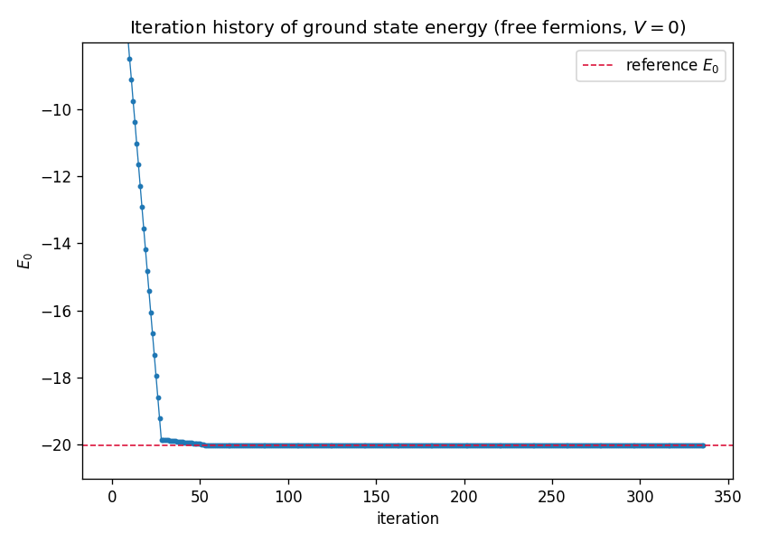
At the DMRG energy reproduces the exact free-fermion value to twelve digits — from a many-body code that has no knowledge that the model is free. The iteration history shows the familiar pattern from DMRG-03: the energy drops steeply during the infinite-system warmup and settles onto its converged value within the first sweep:
Interacting fermions at
MAXSTATES | Truncation error | ||
|---|---|---|---|
| 20 | |||
| 40 | |||
| 60 | |||
| 100 | — |
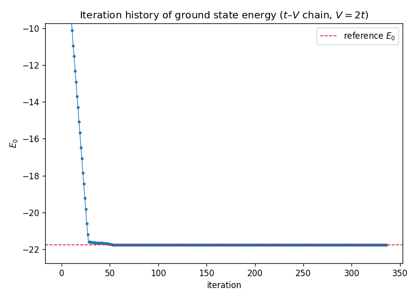
The result agrees with the Jordan–Wigner prediction to every digit of the DMRG-03 reference energy — a direct numerical verification of the operator dictionary derived in the Introduction:
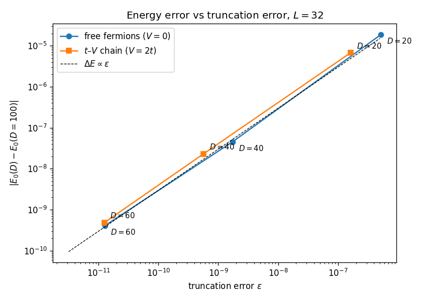
In both cases the energy error is, to a good approximation, proportional to the truncation error — the standard rule of thumb used for extrapolations, which the multiple runs let us check quantitatively:
Summary
DMRG in the particle-number-conserving basis converges the ground state energy of the half-filled spinless-fermion chain essentially to machine precision with states at : the free point reproduces the exact standing-wave energy to twelve digits, and the interacting point reproduces the DMRG-03 Heisenberg energy through the Jordan–Wigner shift to all reported digits, with the energy error scaling linearly in the truncation error in both cases.
Questions
- Fit against the truncation error and extrapolate to . How close is the extrapolated free-fermion energy to the exact value, compared to the raw result?
- Move away from half filling by setting
N_total=8(quarter filling). The free-fermion benchmark is still exact — does the DMRG convergence in get easier or harder, and why? - Scan the interaction across the critical point: keep and compute for . Beyond () the half-filled chain develops charge order — can you detect the transition in the convergence behavior or in the local densities?
- Verify the Jordan–Wigner equivalence end to end on a small chain: run
sparsediagwithMODEL="spinless fermions"and withMODEL="hardcore boson"for , , and confirm that the spectra coincide sector by sector. - Repeat the run without the special-edge chemical potentials (built-in
open chain lattice, uniformmu=1). The result no longer matches the Heisenberg prediction — which term in the bond-by-bond bookkeeping of is responsible for the difference?