DMRG-09 Particle-Number Sectors
Every parameter file in this series has carried the line CONSERVED_QUANTUMNUMBERS="N", and every one has then pinned a single value of N_total and moved on. This module makes the sector itself the variable: the same Hamiltonian, run in three different fixed- blocks, with the energy and the density profile of each read off side by side.
The three lowest blocks are chosen deliberately. They are the only ones on the whole ladder whose answers are known in closed form, which turns them from a physics calculation into a calibration: whatever DMRG returns here can be checked against arithmetic rather than against another simulation.
Phenomena of interest
The symmetry behind the blocks was established in DMRG-07: , so the Hilbert space splits as with , and every eigenstate carries a label . What is new here is the ALPS side of it. Declaring N in CONSERVED_QUANTUMNUMBERS is what tells the code to build those blocks; N_total then selects one. Several { N_total=... } blocks in one parameter file therefore run several independent DMRG calculations whose energies are directly comparable, because they are eigenvalues of one operator.
The step from to is the physical content of this module. It is where a non-interacting problem becomes an interacting one — couples pairs of neighboring sites, so it has nothing to act on below two particles — and both the energy shift and the rearrangement of the density can be measured cleanly, without a thermodynamic-limit extrapolation standing in the way.
In spin language these are the bottom three rungs of the magnetization ladder: the dictionary of DMRG-07 puts at for , so is the magnon density and the profiles below are magnon wavefunctions. DMRG-05 studied the same ladder from its middle, where the interesting structure is at the chain edges; counted from the bottom, the structure is in the bulk.
The model
The – chain, the lattice, and the Jordan–Wigner dictionary are all set up in DMRG-07; nothing about them changes here. Two choices are specific to this module.
No chemical potential. A chemical potential shifts every sector by , which is exactly the term that would make energies from different incomparable. Setting means the numbers in the table below can be subtracted from one another directly.
Two couplings. Every sector is run twice: at for the interacting chain, and at for the free-fermion reference.
Particle sectors
We will study the first three particle sectors. Each is small enough that its answer is known in closed form, which is what makes them a calibration rather than a calculation.
sector: The vacuum is annihilated by every term in , so and on every site, for any and any .
sector: One particle hopping in a box of sites with hard walls. DMRG-08 gives the single-particle eigenstates of the open chain as standing waves , with the ground state energy at filling the sum of the lowest. For one particle that is , and the density profile is a half wavelength:
Both are independent of . This is the sharpest single check in the module: running at and at must give identical numbers, and any difference is a bug rather than physics.
sector: At the two particles fill the two lowest standing waves, , and the density is the sum of the two, — a two-lobed profile with a dip in the middle, which is the hardcore constraint alone keeping the particles apart. At the interaction finally has a pair to act on, and there is no closed form, so this is the one sector of the three whose energy has to be computed rather than written down.
Parameters
| Parameter | Meaning | Value |
|---|---|---|
LATTICE | built-in open chain, no lattice file needed (see the ALPS lattice library) | open chain lattice |
MODEL | hardcore-boson – model, the usable form of the fermion chain (see DMRG-10) | hardcore boson |
CONSERVED_QUANTUMNUMBERS | quantum number held fixed; this is what builds the fixed- blocks | N |
N_total | the block selected — one DMRG run per value | 0, 1, 2 |
L | chain length | 32 |
t | nearest-neighbor hopping amplitude | 1 |
V | nearest-neighbor repulsion | 2 (isotropic point); 0 (free reference) |
mu | chemical potential, omitted so sectors stay comparable | — |
SWEEPS | number of DMRG finite-size sweeps | 6 |
NUMBER_EIGENVALUES | eigenstates requested per sector | 1 |
MAXSTATES | bond dimension kept after truncation | 100 |
MEASURE_LOCAL[...] | site-resolved observable to record | n |
Lattice
The built-in open chain lattice is all that is needed. Every site is equivalent and every bond carries the same and :
      t,V     t,V     t,V                 t,V     t,V
  o-------o-------o-------o  . . .  o-------o-------o
  1       2       3       4         30      31      32

  every bond:  hopping t, interaction V
  every site:  no chemical potential (mu = 0)

  N particles distributed over these 32 sites; N is what N_total fixes
Open boundaries are what make the single-particle levels the clean standing waves used as the reference above — on a ring they would be plane waves with a two-fold degeneracy, and the ground state would not be unique. No lattice file is required.
Choice of method
The dilute sectors are tiny by the standards of this series:
| sector | at |
|---|---|
| 1 | |
| 32 | |
| 496 | |
| (half filling, for contrast) |
Six orders of magnitude separate from the half-filled sector that forced DMRG on us in DMRG-08. That is what makes these blocks a calibration: the answers are known in advance, so the run is being measured rather than trusted. The energies below come from dmrg, each run taking a few seconds at ; the density profiles come from sparsediag, for the reason given under Running the simulation.
Parameter files
The whole module is one parameter file. Each { ... } line is one fixed- block, and the six blocks below cover both couplings, giving six independent runs from a single dmrg invocation — parm_sectors:
LATTICE="open chain lattice"
MODEL="hardcore boson"
CONSERVED_QUANTUMNUMBERS="N"
L=32
t=1
NUMBER_EIGENVALUES=1
SWEEPS=6
MAXSTATES=100
MEASURE_LOCAL[Local density]=n
{ V=2; N_total=0 }
{ V=2; N_total=1 }
{ V=2; N_total=2 }
{ V=0; N_total=0 }
{ V=0; N_total=1 }
{ V=0; N_total=2 }
or equivalently from Python, with sectors.py:
import pyalps
parms = []
for V in [2, 0]:
    for N in [0, 1, 2]:
        parms.append( {
            'LATTICE'                   : 'open chain lattice',
            'MODEL'                     : 'hardcore boson',
            'CONSERVED_QUANTUMNUMBERS'  : 'N',
            'N_total'                   : N,
            'L'                         : 32,
            't'                         : 1,
            'V'                         : V,
            'SWEEPS'                    : 6,
            'NUMBER_EIGENVALUES'        : 1,
            'MAXSTATES'                 : 100,
            'MEASURE_LOCAL[Local density]' : 'n'
        } )
input_file = pyalps.writeInputFiles('parm_sectors',parms)
pyalps.runApplication('dmrg',input_file,writexml=True)
Running the simulation
With the ALPS binaries on your PATH:
parameter2xml parm_sectors
dmrg --write-xml parm_sectors.in.xml
This produces six output files parm_sectors.task1.out.xml … parm_sectors.task6.out.xml, one per block, in the order the blocks appear in the file.
The density profiles need a second run of the same parameters through sparsediag. The legacy ALPS dmrg application measures MEASURE_LOCAL observables only on the final two-site window of the sweep and returns zero on every other site, so it gives energies but not whole-chain profiles. These sectors hold 1, 32 and 496 states, so sparse diagonalization returns the exact profile in under a second — and its energies agree with the DMRG ones to twelve digits, which is the check that licenses mixing the two. Copy the file to a second stem first, so the DMRG results are not overwritten:
cp parm_sectors parm_sectors_ed
parameter2xml parm_sectors_ed
sparsediag --write-xml parm_sectors_ed.in.xml
The script run_number_sectors.py runs the sectors, prints the tables below and draws the figure:
python3 run_number_sectors.py --L 32 --sectors 0 1 2 --plot sectors.pngPass --alps-bin /path/to/alps/bin if the ALPS executables are not on your PATH.
Evaluating the results
Reading the energies and profiles back:
import numpy as np, matplotlib.pyplot as plt, pyalps

# energies from the DMRG run
for run in pyalps.loadEigenstateMeasurements(
        pyalps.getResultFiles(prefix='parm_sectors')):
    N = int(run[0].props['N_total'])
    V = float(run[0].props['V'])
    for s in run:
        if s.props['observable'] == 'Energy':
            print('V = %g, N = %d:  E = %.12f' % (V, N, s.y[0]))

# profiles from the sparsediag run
for run in pyalps.loadEigenstateMeasurements(
        pyalps.getResultFiles(prefix='parm_sectors_ed')):
    N = int(run[0].props['N_total'])
    V = float(run[0].props['V'])
    for s in run:
        if s.props['observable'] == 'Local density' and V == 2:
            y = np.real(np.asarray(s.y).flatten())
            plt.plot(np.arange(1, len(y)+1), y, marker='o', ms=3,
                     label='$N = %d$' % N)
plt.xlabel('site $i$'); plt.ylabel(r'$\langle n_i \rangle$')
plt.legend(); plt.show()
A quick check on any profile run is that recovers N_total; here it does so exactly at every sector.
Energies
, , , six sweeps. The last column is the closed-form free-fermion sum , which is the true answer everywhere except the interacting row:
(dmrg) | exact free-fermion value | |||
|---|---|---|---|---|
| 0 | 1 | |||
| 1 | 32 | |||
| 2 | 496 | |||
| 0 | 1 | |||
| 1 | 32 | |||
| 2 | 496 |
Three things are worth reading off this table.
The blocks are genuinely independent. Six runs came out of one file, and each converged to the ground state of its own sector rather than to the global ground state, which lies far below all of these at half filling (, see DMRG-08).
The check passes. The two rows agree to across a change of the interaction from to , and both reproduce to twelve digits.
carries the interaction energy. Switching on raises the energy from the free value :
It is positive, as a repulsion must be, and small — about of the kinetic energy — because two particles spread over 32 sites are rarely adjacent. It is also far above the noise floor: DMRG resolves a shift of against a total energy of , on a run whose truncation error is .
Density profiles
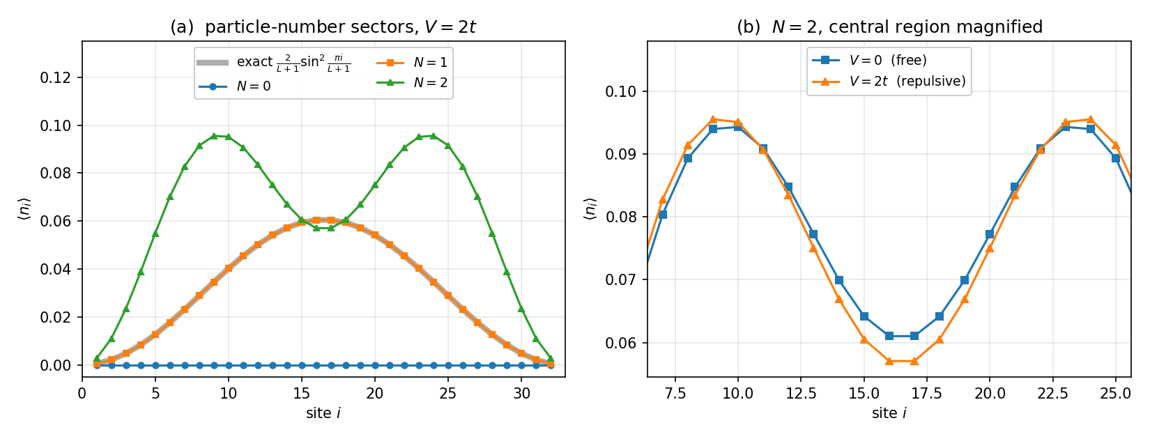
Figure 1. Open chain, , ; profiles from sparsediag, energies from dmrg at . (a) in the three particle-number sectors at , with the exact one-particle standing wave drawn underneath in gray. (b) The profile at and over the central region: the repulsion pushes weight out of the middle of the chain and into the two lobes.
Panel (a) is the three closed forms drawn out. is flat at zero, traces the single standing wave, and shows the two lobes and central dip of — the particles already avoiding each other at , purely because they are hardcore. The curve sits on the analytic profile and does not move between and , which is the check made visible.
Panel (b) isolates what the interaction adds. The two curves lie on top of one another over most of the chain and separate only near the middle — which is where they must. The center is where the two single-particle states overlap most, so it is where the particles are most likely to end up on neighboring sites, and neighboring sites are the only configuration can act on at all. The repulsion therefore costs amplitude precisely there: it suppresses the middle and pushes the weight outward, deepening the dip and raising the two lobes. The split widens, and the particles sit further apart than the hardcore constraint alone would hold them. Nothing is created or destroyed doing it — whatever leaves the center reappears in the lobes.
That last point is exact, and it is worth stating as a check rather than an observation. Every profile here satisfies the particle sum rule:
in every sector and at both couplings, to all reported digits. This is the fermionic face of the spin sum rule used in DMRG-05, — the same statement under the dictionary , and a profile that fails it is not converged in either language.
Qualitatively, this is the same physics that becomes the charge-density-wave transition at once the chain is at half filling and there are enough particles for the avoidance to organize into a pattern. At it is visible in its simplest possible form: two particles and one dip.
Summary
Declaring N conserved turns one Hamiltonian into a ladder of independent blocks, and stacking { N_total=... } lines in a parameter file runs as many of them as you like from a single invocation. In the three dilute blocks the answers are known in closed form, and DMRG reproduces them: in the vacuum, the exact standing-wave energy and profile at for any , and at the first sector where the interaction acts at all — worth in energy and a small redistribution of density out of the chain center.
Questions
- Continue up the ladder: add
{ V=2; N_total=3 }and{ V=2; N_total=4 }. The interaction energy grows with — does it grow like , like , or like something else, and what does that say about how often two particles are adjacent? - Build the chemical potential back in. The addition energy is what it costs to put one more particle on the chain. Compute it for and check that at it reproduces the single-particle levels exactly.
- Make attractive. Set at : two particles now gain energy by sitting next to each other. Does the density profile develop a peak at the chain center instead of a dip, and can you find the threshold at which a two-particle bound state forms?
- Check the spin dictionary directly. Run the same three sectors as
MODEL="spin"withSz_totalat , , and confirm that the energies differ from the ones above only by the constant derived in DMRG-11. - Push the sector until DMRG has to work. Repeat at and with and : at which filling do the two bond dimensions first disagree, and how does that track the Hilbert-space dimensions in the table above?