ED-02 Gaps
Spin gaps of 1D quantum spin systems
In this tutorial we will use the sparse diagonalization program to compute spin gaps of 1D quantum spin systems and study their finite-size scaling. A central question for any antiferromagnetic spin chain is whether it has a finite excitation gap above its ground state, or is gapless. Haldane conjectured — and it is now firmly established, both numerically and by field-theoretic arguments — that isotropic Heisenberg chains behave completely differently depending on whether the spin quantum number is an integer or a half-integer: integer-spin chains have a unique, gapped ground state (the “Haldane gap”), while half-integer-spin chains are gapless with power-law-decaying correlations (F.D.M. Haldane, Phys. Rev. Lett. 50, 1153 (1983)). Because a finite system always has a discrete spectrum, this qualitative difference only becomes visible after extrapolating the finite-size gap to — which is exactly what we do below for and .
The Hamiltonian in both cases is the isotropic Heisenberg chain:
on a periodic chain of sites, differing only in the local spin length .
Parameters
| Parameter | Meaning | Value |
|---|---|---|
LATTICE | periodic chain | chain lattice |
MODEL | quantum spin model | spin |
local_S | spin quantum number per site | 1 (parm2a) or 1/2 (parm2b) |
J | nearest-neighbor Heisenberg coupling | 1 |
L | chain length | 4, 6, 8, 10 |
CONSERVED_QUANTUMNUMBERS | symmetry used to block-diagonalize | Sz |
Sz_total | restricts the diagonalization to a single sector | 0 (singlet sector) and 1 (triplet sector) |
Lattice
Both chains use the built-in periodic chain lattice from the ALPS lattice library, sketched here for :
    J       J       J       J       J
o-------o-------o-------o-------o-------o
0       1       2       3       4       5
|_______________________________________|
                   J   (bond 5-0, periodic)
Method
Diagonalizing separately in the and sectors and taking the lowest eigenvalue of each isolates the singlet ground state and the lowest triplet excitation without having to search through the (much larger) full spectrum. Even the largest sector here (, , dimension ) is easily handled by the Lanczos iteration behind sparsediag; full diagonalization would be unnecessary and considerably more expensive since we only need the lowest state in each sector.
Spin gap of a spin-1 chain
Using the command line
The parameter file parm2a sets up exact diagonalization of the quantum mechanical S=1 chain with 4 to 10 sites in the singlet and triplet sector:
MODEL="spin"
LATTICE="chain lattice"
CONSERVED_QUANTUMNUMBERS="Sz"
local_S=1
J=1
Sz_total=0
{L=4}
{L=6}
{L=8}
{L=10}
Sz_total=1
{L=4}
{L=6}
{L=8}
{L=10}
The parameter Sz_total restricts the conserved quantum number Sz to the given value. See the model library documentation for more details on how to set up models and conserved quantum numbers.
Using the standard sequence of commands you can first convert the input parameters to XML and then run the application sparsediag:
parameter2xml parm2a
sparsediag --write-xml parm2a.in.xml
Evaluation of the gaps can now be done manually by looking at the output files, or we can use Python to automate the whole workflow.
Using Python
To set up and run the simulation in Python we use the script tutorial2a.py. The first parts of this script imports the required modules, prepares the input files as a list of Python dictionaries, writes the input files and runs the application:
import pyalps
import numpy as np
import matplotlib.pyplot as plt
import pyalps.pyplot
parms = []
for l in [4, 6, 8, 10]:
    for sz in [0, 1]:
        parms.append({
            'LATTICE'                   : "chain lattice",
            'MODEL'                     : "spin",
            'local_S'                   : 1,
            'J'                         : 1,
            'L'                         : l,
            'CONSERVED_QUANTUMNUMBERS'  : 'Sz',
            'Sz_total'                  : sz
        })

input_file = pyalps.writeInputFiles('parm2a',parms)
res = pyalps.runApplication('sparsediag',input_file)
To run this, in your terminal type python tutorial2a.py. We now have the same output files as in the command line version.
We next load the spectra for each of the systems sizes and spin sectors:
data = pyalps.loadSpectra(pyalps.getResultFiles(prefix='parm2a'))To extract the gaps we need to write a few lines of Python, to set up a list of lengths and a Python dictionaries of the minimum energy in each (L,Sz) sector:
lengths = []
min_energies = {}
for sim in data:
    l = int(sim[0].props['L'])
    if l not in lengths: lengths.append(l)
    sz = int(sim[0].props['Sz_total'])
    all_energies = []
    for sec in sim:
        all_energies += list(sec.y)
    min_energies[(l,sz)]= np.min(all_energies)
And finally we make a plot of the gap as a function of 1/L and then show the plot:
gapplot = pyalps.DataSet()
gapplot.x = 1./np.sort(lengths)
gapplot.y = [min_energies[(l,1)] -min_energies[(l,0)] for l in np.sort(lengths)]
gapplot.props['xlabel']='$1/L$'
gapplot.props['ylabel']='Triplet gap $\Delta/J$'
gapplot.props['label']='S=1'

plt.figure()
pyalps.plot.plot(gapplot)
plt.legend()
plt.xlim(0,0.25)
plt.ylim(0,1.0)
plt.show()
Spin gap of a spin-1/2 chain
Compare the extrapolated gap of the spin-1 chain to that of a spin-1/2 chain. To do so, just change the local spin local_S=1 to local_S=0.5 and run the simulations (but give them the name parm2b). The parameter file parm2b is otherwise identical to parm2a:
MODEL="spin"
LATTICE="chain lattice"
CONSERVED_QUANTUMNUMBERS="Sz"
local_S=1/2
J=1
Sz_total=0
{L=4}
{L=6}
{L=8}
{L=10}
Sz_total=1
{L=4}
{L=6}
{L=8}
{L=10}
The Python script is tutorial2b.py.
Both systems in one plot
To show both gaps in one plot run the Python script tutorial2c.py after running the first two tutorials.
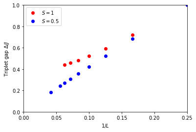
The gaps as a function of lattice size for both spin 1/2 and 1 are plotted in the following figure:
Output data
The table below lists the exact triplet gap obtained from the two parameter files, for reference against your own run:
| Gap , S=1 | Gap , S=1/2 | ||
|---|---|---|---|
| 4 | 0.250 | 1.0000 | 1.0000 |
| 6 | 0.167 | 0.7206 | 0.6847 |
| 8 | 0.125 | 0.5936 | 0.5227 |
| 10 | 0.100 | 0.5248 | 0.4232 |
The S=1 gap is leveling off and extrapolates (e.g. by a quadratic fit in ) to a finite value close to the literature estimate for the Haldane gap, , while the S=1/2 gap keeps decreasing and is consistent with extrapolating to zero — the hallmark of a gapless chain.
Summary
For the same nearest-neighbor antiferromagnetic Heisenberg coupling, the S=1 chain extrapolates to a finite excitation gap while the S=1/2 chain extrapolates to zero, directly confirming the Haldane conjecture on chains small enough to diagonalize exactly.
Questions
- What is the extrapolated value of the gap for an infinite system?
- Why do the S=1/2 and S=1 chains show different behavior?
- Try a quadratic fit to the S=1 data in the table above. How close is your extrapolated to the literature value of ?