ED-03 Spectra

Energy Spectra of 1D quantum systems

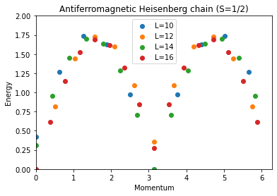
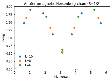
In this tutorial we will calculate the energy spectra of the quantum Heisenberg model on various one-dimensional lattices. The main work will be done by the sparsediag application, which implements the Lanczos algorithm, an iterative eigensolver. Unlike the ground-state and gap calculations of the previous tutorials, here we compute several low-lying eigenvalues in every momentum sector, so that we can assemble the full momentum-resolved excitation spectrum $E(k)$. This is the basic diagnostic used to identify what kind of excitations a model has — a single dispersing magnon branch, a two-spinon continuum, gapped triplon bound states — simply by looking at the shape of the low-energy spectrum as a function of lattice geometry and coupling.

All three examples below (chain, ladder, isolated dimers) are special cases of the same Heisenberg Hamiltonian on a two-leg ladder,

where $J_0$ is the coupling along the two legs and $J_1$ the coupling across the rungs; setting $J_0=J_1$ gives the isotropic ladder, $J_1=0$ gives two decoupled chains, and $J_0=0$ gives $L$ isolated two-site dimers. This family of models, and the crossover between its limits, is discussed e.g. in E. Dagotto and T.M. Rice, Science 271, 618 (1996).

Parameters

Method

We use sparsediag because we need not just the ground state but several of the lowest eigenvalues in every momentum sector to build up $E(k)$; the Lanczos algorithm computes any requested number of extremal eigenvalues of a sparse Hamiltonian directly, without diagonalizing sectors we are not interested in. The largest sector here (chain, $L=16$, $S_z=0$) has dimension $\binom{16}{8}=12870$, comfortably within reach of iterative sparse diagonalization while being far too large to enumerate by hand.

Heisenberg chain

The chain lattice (built into the ALPS lattice library) is a periodic ring of $L$ sites with uniform coupling $J$:

    J     J     J           J
o-------o-------o--- ... ---o
0       1       2          L-1
|_________________________________|
                J   (bond L-1 -- 0, periodic)

Preparing and running the simulation from the command line

First, we look at a chain of S=1/2 spins with Heisenberg coupling. The parameter file parm_chain sets up ED simulations for the S_z=0 sector of chains with {L=10,…16} spins.

LATTICE = "chain lattice", 
MODEL = "spin",
local_S = 0.5,
J = 1,
CONSERVED_QUANTUMNUMBERS = "Sz"
Sz_total = 0
{ L = 10; }
{ L = 12; }
{ L = 14; }
{ L = 16; }

Using the following sequence of commands you can run the diagonalization, then look at the output file parm_chain.out.xml with your browser.

parameter2xml parm_chain
sparsediag --write-xml parm_chain.in.xml

Preparing and running the simulation using Python

To set up and run the simulation in Python, we use the script chain.py. You can run it in a terminal with python chain.py. Looking at the different parts of the script, we see how the input files are prepared as a list of Python dictionaries after importing the required modules.

import pyalps
import numpy as np
import matplotlib.pyplot as plt
import pyalps.plot

parms=[]
for l in [10, 12, 14, 16]:
    parms.append({ 
        'LATTICE'                   : "chain lattice", 
        'MODEL'                     : "spin",
        'local_S'                   : 0.5,
        'J'                         : 1,
        'L'                         : l,
        'CONSERVED_QUANTUMNUMBERS'  : 'Sz',
        'Sz_total'                  : 0
    })

Next, the input parameters are written into XML job files and the sparsediag simulation is run.

input_file = pyalps.writeInputFiles('parm_chain',parms)
res = pyalps.runApplication('sparsediag',input_file)

For plotting the spectrum, we then load the HDF5 files produced by the simulation

data = pyalps.loadSpectra(pyalps.getResultFiles(prefix='parm_chain'))

and collect the energies from all momentum sectors into one DataSet for each system size L. For getting a nice plot we additionally subtract the ground state energy from all eigenvalues and assign a label and line style to each spectrum.

spectra = {}
for sim in data:
    l = int(sim[0].props['L'])
    all_energies = []
    spectrum = pyalps.DataSet()
    for sec in sim:
        all_energies += list(sec.y)
        spectrum.x = np.concatenate((spectrum.x,np.array([sec.props['TOTAL_MOMENTUM'] for i in range(len(sec.y))])))
        spectrum.y = np.concatenate((spectrum.y,sec.y))
        spectrum.y -= np.min(all_energies)
    spectrum.props['line'] = 'scatter'
    spectrum.props['label'] = 'L='+str(l)
    spectra[l] = spectrum

Now the spectra from different system sizes can be plotted into one figure:

plt.figure()
pyalps.plot.plot(spectra.values())
plt.legend()
plt.title('Antiferromagnetic Heisenberg chain (S=1/2)')
plt.ylabel('Energy')
plt.xlabel('Momentum')
plt.xlim(0,2*3.1416)
plt.ylim(0,2)
plt.show()

The plotted energy spectra for the Heisenberg chain is shown below:

Two-leg Heisenberg ladder

With only a few small changes to the input parameters used above, we can calculate the spectrum of a two-leg ladder of Heisenberg spins. The ladder lattice places $2L$ sites in two rows of $L$, connected by leg bonds $J_0$ and rung bonds $J_1$:

o---J0---o---J0---o---...---o     leg 0
|        |        |         |
J1       J1       J1        J1
|        |        |         |
o---J0---o---J0---o---...---o     leg 1

The new parameter text file parm_ladder looks like this:

LATTICE = "ladder"
MODEL = "spin"
local_S = 0.5
J0 = 1
J1 = 1
CONSERVED_QUANTUMNUMBERS = "Sz"
Sz_total = 0
{ L = 6; }
{ L = 8; }
{ L = 10; }

We have just replaced the “chain lattice” by a “ladder” and defined two separate coupling constants J0, J1 for the legs and the rungs, respectively. Apart from that, we have reduced the linear system size L because the ladder has 2L spins. Run it exactly as before:

parameter2xml parm_ladder
sparsediag --write-xml parm_ladder.in.xml

The same changes have to be made to the Python code, which can be downloaded from here: ladder.py

The energy spectra of a Heisenberg ladder for various lattice sizes are shown below:

Isolated dimers

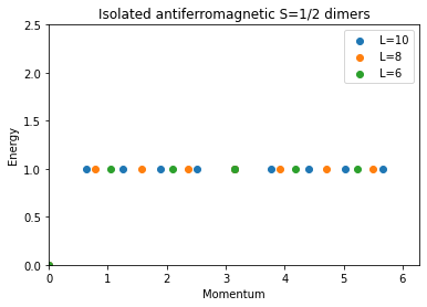
If we set the coupling on the legs of the ladder J0 = 0, we get the spectrum of L isolated dimers — each rung decouples into an independent two-site singlet/triplet problem, so the “spectrum” collapses to just two exactly degenerate levels (a singlet at $E=-3J_1/4$ and a flat triplet band at $E=+J_1/4$) for every value of the momentum. This is done in the parameter file parm_dimers:

LATTICE = "ladder"
MODEL = "spin"
local_S = 0.5
J0 = 0
J1 = 1
CONSERVED_QUANTUMNUMBERS = "Sz"
Sz_total = 0
{ L = 6; }
{ L = 8; }
{ L = 10; }

and the Python script dimers.py. Run it the same way:

parameter2xml parm_dimers
sparsediag --write-xml parm_dimers.in.xml

The energy spectra of isolated dimers are presented in the following

Summary

Turning a single coupling constant ($J_0$) on and off morphs the excitation spectrum continuously from a dispersionless flat band (isolated dimers) through a two-branch spectrum with a bound-state/continuum structure (the ladder) to the gapless two-spinon continuum of the single chain — illustrating how spectral shape alone reveals the nature of a system’s low-energy excitations.

Questions

• Observe how putting together spectra from different system sizes produces nice bands
• In the spectrum of the Heisenberg ladder: Identify continuum and bound states
• What is the major difference between the chain and the ladder spectrum?
• Explain the spectrum of isolated dimers
• Vary the coupling constants in the ladder and observe how the spectrum changes between the limits discussed before
• Bonus question: Have a close look at the spectrum of the chain for different system sizes: There seems to be a difference between cases where L/2 is even and those where it is odd. Can you explain this? What happens in the TDL where L goes to infinity?