DMFT of Hubbard Model on a Bethe Lattice
The dynamical mean-field theory (DMFT) for strongly correlated electron systems is based on mapping of lattice models onto quantum impurity models subject to a self-consistency condition A. Georges, G. Kotliar, W. Krauth, and M.J. Rozenberg, Reviews of Modern Physics 68, 13-125 (1996). The mapping is exact for models of correlated electrons in the limit of large lattice coordination or infinite spatial dimensions. Bethe lattice is an example lattice with infinite spatial dimensions and can be simulated by DMFT with ALPS.
Bethe Lattice
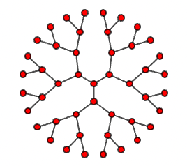
An example picture of Bethe lattice is shown below, where there are 3 coordination numbers for each lattice site. The effective dimension of the lattice is infinite. It, therefore, offers a great opportunity to implement DMFT on such a lattice, where the DMFT method can be benchmarked and explored.
Hubbard Model
We will simulate Hubbard model defined on a Bethe lattice with DMFT. The Hubbard model is defined below.
where
- and are creation and annihilation operators for a fermion with flavor (up or down ) at site and represents Hermitian Conjugate.
- is hopping amplitude between neighboring sites .
- is on-site interaction energy, with corresponding to repulsive interactions.
- is number operator for fermions with flavor at site .
Parameters
| Parameter | Meaning | Value |
|---|---|---|
SOLVER | impurity solver algorithm | Interaction Expansion (CT-INT QMC) |
U | on-site Hubbard repulsion | 3 |
t | hopping amplitude, rescaled for the Bethe lattice | 0.707106781... () |
BETA | inverse temperature | 6 (high ), 12 (low ) |
MU | chemical potential (half filling) | 0 |
FLAVORS | number of fermion flavors (spin up/down) | 2 |
SITES | number of impurity sites | 1 |
ANTIFERROMAGNET | allow symmetry-broken AFM solution | 1 |
H_INIT | initial symmetry-breaking field, to seed the AFM state | 0.05 |
N, NMATSUBARA | number of imaginary-time / Matsubara-frequency points | 500 |
SWEEPS, THERMALIZATION | QMC sweeps and thermalization steps | 1e8, 1000 |
MAX_IT, MAX_TIME | DMFT self-consistency iterations, wall-time cap per iteration (s) | 10, 10 |
CONVERGED | self-consistency convergence threshold | 0.005 |
Lattice
        o   o
         \ /
      o---o---o        each site has z=3 neighbours,
         / \            connected in a loop-free tree
        o   o            → Bethe lattice, coordination z=3
The Bethe lattice (an infinite, loop-free tree) is used because it is the simplest lattice for which DMFT becomes numerically exact in the limit of infinite coordination number — the self-consistency condition for the local Green’s function collapses to the simple semicircular-DOS relation used internally by pyalps.runDMFT, with the hopping rescaled by (hence t=1/sqrt(2) for effective coordination in the infinite- limit) so the bandwidth stays finite. See the ALPS lattice library for finite-dimensional lattices where DMFT is instead an approximation.
Method Choice
Unlike the ED/DMRG tutorials, the local impurity problem here is solved stochastically: the Interaction Expansion continuous-time quantum Monte Carlo (CT-INT) solver samples diagrams in powers of rather than diagonalizing a Hamiltonian, which is what makes it possible to reach the true infinite-coordination Bethe lattice (no finite-size Hilbert space to truncate). MAX_TIME=10 caps each DMFT iteration to 10 seconds of QMC sampling regardless of the nominal SWEEPS=1e8, so the full MAX_IT=10-iteration self-consistency loop for both temperatures completes in a few minutes.
Simulation
We first import the required modules.
import pyalps
import numpy as np
import matplotlib.pyplot as plt
import pyalps.plot
Then we prepare the input files as a list of Python dictionaries.
parms=[]
for b in [6., 12.]:
    parms.append(
            {
              'ANTIFERROMAGNET'         : 1,
              'CONVERGED'               : 0.005,
              'FLAVORS'                 : 2,
              'H'                       : 0,
              'H_INIT'                  : 0.05,
              'MAX_IT'                  : 10,
              'MAX_TIME'                : 10,
              'MU'                      : 0,
              'N'                       : 500,
              'NMATSUBARA'              : 500,
              'OMEGA_LOOP'              : 1,
              'SEED'                    : 0,
              'SITES'                   : 1,
              'SOLVER'                  : 'Interaction Expansion',
              'SYMMETRIZATION'          : 0,
              'U'                       : 3,
              't'                       : 0.707106781186547,
              'SWEEPS'                  : 100000000,
              'THERMALIZATION'          : 1000,
              'ALPHA'                   : -0.01,
              'HISTOGRAM_MEASUREMENT'   : 1,
              'BETA'                    : b
            }
        )
The parameter “BETA” refers to inverse temperature and we are simulating the system at two different temperatures, “BETA = 6” at high temperature and “BETA = 12” at low temperature. We then write the input file and run the simulation.
for p in parms:
    input_file = pyalps.writeParameterFile('parm_beta_'+str(p['BETA']),p)
    res = pyalps.runDMFT(input_file)
We next load the result of the simulation.
listobs=['0', '1']

data = pyalps.loadMeasurements(pyalps.getResultFiles(pattern='parm_beta_*h5'), respath='/simulation/results/G_tau', what=listobs)
for d in pyalps.flatten(data):
    d.x = d.x*d.props["BETA"]/float(d.props["N"])
    d.props['label'] = r'$\beta=$'+str(d.props['BETA'])+'; flavor='+str(d.props['observable'][len(d.props['observable'])-1])
And finally we make a plot of the single-particle Green’s function vs. the imaginary time and then show the plot.
plt.figure()
plt.xlabel(r'$\tau$')
plt.ylabel(r'$G_{flavor}(\tau)$')
plt.title("Green's Function vs. the Imaginary Time")
pyalps.plot.plot(data)
plt.legend()
plt.show()
The graph of the simulation should look like below:
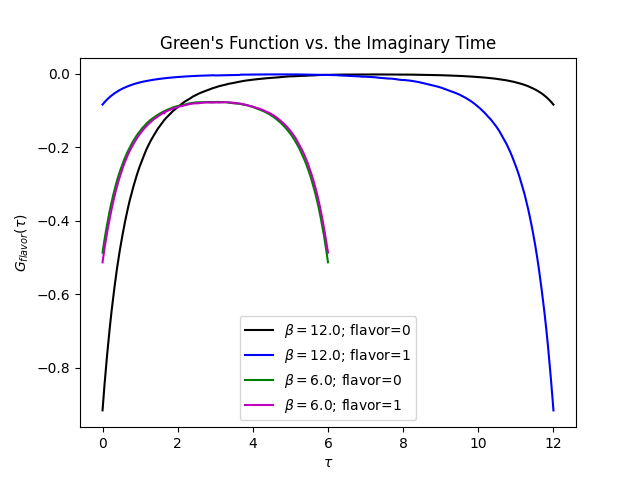
The result shows a Neel transition for the Hubbard model on the Bethe lattice, where the system undergoes a transition from the antiferromagnetic state at low temperatures (“BETA = 12”) to the paramagnetic state at high temperatures (“BETA = 6”).
Results
The single-particle Green’s function at the two ends of the imaginary-time interval, from running the code above:
| Flavor | |||
|---|---|---|---|
| 6 | 0 (↑) | -0.4868 | -0.0759 |
| 6 | 1 (↓) | -0.5132 | -0.0776 |
| 12 | 0 (↑) | -0.8932 | -0.0039 |
| 12 | 1 (↓) | -0.1066 | -0.0037 |
At , the two spin flavors are nearly symmetric ( vs. ) — a paramagnetic solution. At , the flavors split strongly ( vs. ) — the AFM symmetry-breaking field H_INIT has grown into a robust staggered magnetization, signalling the system has crossed into the antiferromagnetically-ordered phase on cooling.
Summary and Outlook
DMFT on the Bethe lattice shows the half-filled Hubbard model crossing from a paramagnetic solution at high temperature () to a magnetically-ordered (Néel) solution at low temperature (), visible directly in the splitting of the two spin flavors’ Green’s functions.
- At what value of between 6 and 12 does the splitting between the two flavors first become significant — can you bracket the Néel transition temperature?
- How does the transition temperature shift if the interaction is increased from 3 to 6?
- What would you expect to see in the paramagnetic phase if you additionally computed the local density of states via
maxent?