Extrapolation of Energy Gap for a Spin-1/2 Chain
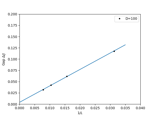
In this tutorial, we will calculate energy gap for a spin-1/2 chain with various lattice sizes: 32, 64, 96, and 128. We will fix the number of states in the DMRG simulation to , which produces results with enough accuracy. The energy gaps vs lattice sizes will be plotted and extrapolated to the thermodynamic limit.
The Hamiltonian is the antiferromagnetic Heisenberg exchange model, first introduced by W. Heisenberg, Zeitschrift für Physik 49, 619-636 (1928):
For a spin-1/2 chain, the gap is known to close as in the thermodynamic limit, which is the scaling form fitted below.
Parameters
| Parameter | Meaning | Value |
|---|---|---|
LATTICE | lattice used for the chain | open chain lattice |
MODEL | Hamiltonian family | spin |
CONSERVED_QUANTUMNUMBERS | quantum numbers fixed in the basis | Sz |
Sz_total | total magnetization sector | 0 |
J | Heisenberg exchange coupling | 1 |
SWEEPS | number of DMRG sweeps | 4 |
L | chain length | 32, 64, 96, 128 |
MAXSTATES | number of DMRG basis states kept | 100 |
NUMBER_EIGENVALUES | number of low-lying eigenstates kept | 2 |
Lattice
   J     J     J             J
o-----o-----o-----o-- ... --o     (L = 32, 64, 96, or 128 sites, open boundary conditions)
Same open chain lattice as the single-size gap tutorial, repeated at four lengths so the finite-size gap can be extrapolated to . See the ALPS lattice library for other built-in lattices.
Method Choice
At the untruncated Hilbert space is , astronomically beyond exact diagonalization; DMRG with a fixed MAXSTATES=100 keeps the calculation tractable at every size while still resolving the gap accurately enough for the extrapolation below. All four sizes together run in well under a minute.
We first import the necessary libraries.
import pyalps
import numpy as np
import matplotlib.pyplot as plt
import pyalps.plot
import pyalps.fit_wrapper as fw
We prepare the input files with various lattice sizes for multiple runs.
parms= []
for lattice in [32, 64, 96, 128]:
    parms.append({
            'LATTICE'                   : "open chain lattice",
            'MODEL'                     : "spin",
            'CONSERVED_QUANTUMNUMBERS'  : 'Sz',
            'Sz_total'                  : 0,
            'J'                         : 1,
            'SWEEPS'                    : 4,
            'L'                         : lattice,
            'MAXSTATES'                 : 100,
            'NUMBER_EIGENVALUES'        : 2
        })
Notice that we have set the maximum number of states to be kept in the DMRG simulations. The lowest two eigin values will be kept and used to calculate the energy gap.
We then write the input files and run the simulations.
input_file = pyalps.writeInputFiles('parm_spin_one_half_gap_multiple',parms)
res = pyalps.runApplication('dmrg',input_file,writexml=True)
After the simulations, we load all measurements for all lattices and sort the results according to the lattice sizes.
data = pyalps.loadEigenstateMeasurements(pyalps.getResultFiles(prefix='parm_spin_one_half_gap_multiple'))

sorted_data = sorted(data, key=lambda x: x[0].props['L'])
A data set is created for the pyalps plot function. The energy gaps for each lattice size are also included in the data set.
gapplot = pyalps.DataSet()
gapplot.props['xlabel']='$1/L$'
gapplot.props['ylabel']='Gap $\Delta/J$'
gapplot.props['label']='D=100'
gapplot.props['line']='.'

x = []
y = []
for measure in sorted_data:
    for s in measure:
        if s.props['observable'] == 'Energy':
            L = s.props['L']
            iL = 1.0/L
            gap = abs(s.y[1] - s.y[0])
            s.props['gap'] = gap
            x.append(iL)
            y.append(gap)

gapplot.x = x
gapplot.y = y
We plot the energy gap vs 1/L relation, which is fitted with a linear curve. The fitted curve is also plotted in the same figure.
# plot the gap vs. 1/L curve:
plt.figure()
pyalps.plot.plot(gapplot)
plt.legend()
plt.xlim(0,0.04)
plt.ylim(0,0.2)

# fit the curve with a linear function
pars = [fw.Parameter(0.1), fw.Parameter(0.2)]
f = lambda self, x, p: p[0]()+p[1]()*x
fw.fit(None, f, pars, np.array(gapplot.y), np.array(gapplot.x))

# plot the fitted curve
x = np.linspace(0.0, 0.035, 100)
plt.plot(x, f(None,x,pars))

print("Gap at thermodynamic limit: ", pars[0]())

plt.show()
The final energy gap figure should look like the following:
Results
Running the code above gives:
| Gap | ||
|---|---|---|
| 32 | 0.03125 | 0.11774 |
| 64 | 0.01563 | 0.06176 |
| 96 | 0.01042 | 0.04205 |
| 128 | 0.00781 | 0.03194 |
The linear fit in extrapolates to at — consistent with zero within the fit’s finite-size systematic error, confirming that the spin-1/2 Heisenberg chain is gapless.
Summary and Outlook
The DMRG-computed gap for the spin-1/2 Heisenberg chain shrinks approximately linearly in and extrapolates to essentially zero, confirming the chain is gapless in the thermodynamic limit — in direct contrast to the finite Haldane gap found for the spin-1 chain.
- Is a strictly linear fit in the best choice here, or would a form with logarithmic corrections (as predicted by field theory for the spin-1/2 chain) fit better?
- How does the extrapolated gap change if you include larger lattice sizes, e.g. ?
- Compare this extrapolation to the spin-1 case: why does that one extrapolate to a finite gap instead of zero?