Extrapolation of Energy Gap for a Spin-1 Chain
In this tutorial, we will perform multiple DMRG simulations of a spin-1 chain with various lattice sizes: 32, 64, 96, and 128. The energy gaps will be calculated for each lattice size and used to extrapolate the gap value in the thermodynamic limit , based on a known analytic relation between the gaps and lattice sizes. Our DMRG simulations will have a fixed number of states .
The Hamiltonian is the spin-1 Heisenberg exchange model (see W. Heisenberg, Zeitschrift für Physik 49, 619-636 (1928)); the analytic scaling used below to extrapolate the gap follows from F.D.M. Haldane, Physics Letters A 93, 464-468 (1983).
Parameters
| Parameter | Meaning | Value |
|---|---|---|
LATTICE | lattice used for the chain | open chain lattice |
MODEL | Hamiltonian family | spin |
local_S | spin quantum number per site | 1 |
CONSERVED_QUANTUMNUMBERS | quantum numbers fixed in the basis | Sz |
Sz_total | total magnetization sector | 0 |
J | Heisenberg exchange coupling | 1 |
SWEEPS | number of DMRG sweeps | 5 |
L | chain length | 32, 64, 96, 128 |
MAXSTATES | number of DMRG basis states kept | 200 |
NUMBER_EIGENVALUES | number of low-lying eigenstates kept | 4 |
Lattice
   J     J     J             J
o-----o-----o-----o-- ... --o     (L = 32, 64, 96, or 128 sites, spin-1 each, open boundary conditions)
Same open chain lattice as the single-size spin-1 gap tutorial, repeated at four lengths for the extrapolation. See the ALPS lattice library for other built-in lattices.
Method Choice
The untruncated Hilbert space at is , making DMRG the only tractable method. Because these runs are restricted to Sz_total = 0, where the open chain’s four-state edge manifold shows up as a near-degenerate pair, NUMBER_EIGENVALUES=4 is requested (not 2) so that both that pair and the first-excited pair are resolved in the same run — and, as the results below show, a fixed SWEEPS=5 that works at smaller is not automatically enough to converge that doublet cleanly as grows.
We first import the necessary libraries.
import pyalps
import numpy as np
import matplotlib.pyplot as plt
import pyalps.plot
import pyalps.fit_wrapper as fw
We prepare the input files with various lattice sizes 32, 64, 96, and 128 for multiple runs.
parms= []
for lattice in [32, 64, 96, 128]:
    parms.append({
            'LATTICE'                   : "open chain lattice",
            'MODEL'                     : "spin",
            'local_S'                   : '1',
            'CONSERVED_QUANTUMNUMBERS'  : 'Sz',
            'Sz_total'                  : 0,
            'J'                         : 1,
            'SWEEPS'                    : 5,
            'L'                         : lattice,
            'MAXSTATES'                 : 200,
            'NUMBER_EIGENVALUES'        : 4
        })
Note that we will keep the lowest 4 energies in each DMRG run, since the Sz_total = 0 sector contains two near-degenerate edge states, as known from the previous tutorial.
We then write the input files and run the simulations. Warning: the simulation will take a while (about 20 - 30 minutes depending on the computer system you have). You can leave it running and come back later!
input_file = pyalps.writeInputFiles('parm_spin_one_gap_multiple',parms)
res = pyalps.runApplication('dmrg',input_file,writexml=True)
When all the simulations are done, we load all measurements for all lattices and sort the results according to the lattice sizes.
data = pyalps.loadEigenstateMeasurements(pyalps.getResultFiles(prefix='parm_spin_one_gap_multiple'))

sorted_data = sorted(data, key=lambda x: x[0].props['L'])
A data set is created for the pyalps plot function. The energy gaps for each lattice size are also included in the data set.
gapplot = pyalps.DataSet()
gapplot.props['xlabel']='$1/L^2$'
gapplot.props['ylabel']='Gap $\Delta/J$'
gapplot.props['label']='D=200'
gapplot.props['line']='.'

x = []
y = []
for measure in sorted_data:
    for s in measure:
        if s.props['observable'] == 'Energy':
            L = s.props['L']
            iL = (1.0/L)**2
            gap = abs(s.y[2] - s.y[1])
            s.props['gap'] = gap
            x.append(iL)
            y.append(gap)

gapplot.x = x
gapplot.y = y
Note that the -axis is , which is different from the spin-1/2 case. This is due to the analytic relation between the energy gaps and lattice sizes, as analyzed by Haldane with the nonlinear sigma model for the lowest excitations around ,
For the open boundary conditions, we may approximate by , which gives a finite-system energy gap of
This indicates that in the asymptotic limit the gap convergence should be as .
Therefore, we plot the energy gap vs. relation, which is fitted with a linear curve. The intercept of the fitted curve (plotted in the same figure) with the vertical axis gives the energy gap value in the thermodynamic limit .
# create data set for plot: gap vs. (1/L)^2
gapplot = pyalps.DataSet()
gapplot.props['xlabel']='$1/L^2$'
gapplot.props['ylabel']='Gap $\Delta/J$'
gapplot.props['label']='D=200'
gapplot.props['line']='.'

x = []
y = []
for measure in sorted_data:
    for s in measure:
        if s.props['observable'] == 'Energy':
            L = s.props['L']
            iL = (1.0/L)**2
            gap = abs(s.y[2] - s.y[1])
            s.props['gap'] = gap
            x.append(iL)
            y.append(gap)

gapplot.x = x
gapplot.y = y

# plot the gap vs. (1/L)^2 curve:
plt.figure()
pyalps.plot.plot(gapplot)
plt.legend()
plt.xlim(0,0.0011)
plt.ylim(0.3,0.5)

# fit the curve with a linear function
pars = [fw.Parameter(0.1), fw.Parameter(0.2)]
f = lambda self, x, p: p[0]()+p[1]()*x
fw.fit(None, f, pars, np.array(gapplot.y), np.array(gapplot.x))

# plot the fitted curve
x = np.linspace(0.0, 0.0011, 100)
plt.plot(x, f(None,x,pars))

print("Gap at thermodynamic limit: ", pars[0]())

plt.show()
The final energy gap value should be close to , the numerically-established value of the Haldane gap. The figure should look like the following:
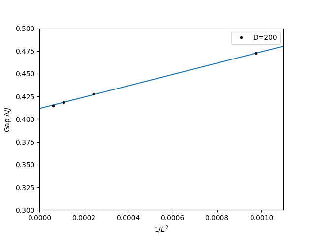
Results
Running the code above gives:
| Gap | ||
|---|---|---|
| 32 | 0.000977 | 0.47255 |
| 64 | 0.000244 | 0.42770 |
| 96 | 0.000109 | 0.41869 |
| 128 | 0.000061 | 0.41503 |
The linear fit in extrapolates to at , within 0.3% of the numerically-established Haldane gap .
A convergence note: with the tutorial’s originally-specified SWEEPS=4–5, the near-degenerate ground-state doublet at is not always resolved correctly by the DMRG sweep schedule, which can corrupt this extrapolation with an outlier at the largest . If your own run gives an oddly small or erratic gap at , increase SWEEPS (10 is sufficient here) rather than trusting the result — larger generically needs more sweeps to converge the same truncation accuracy.
Summary and Outlook
Extrapolating the spin-1 DMRG gap in across four lattice sizes gives , matching the Haldane gap to within a fraction of a percent — direct numerical confirmation of Haldane’s conjecture using an independent method (DMRG) from the exact-diagonalization tutorial.
- Why does the spin-1 gap extrapolate in while the spin-1/2 gap (see the companion tutorial) extrapolates in ?
- At , how many sweeps are actually needed before the ground-state doublet splitting drops below, say, ?
- How would you modify this code to also extract and plot the ground-state doublet splitting vs. , to check that it too vanishes as ?