Transverse Field Quantum Ising Model
Introduction
In this tutorial, we will look at critical spin chains and make a connection to their description in terms of conformal field theory.
The model we will consider is the critical Ising chain, given by the Hamiltonian
Here, the first sum runs over pairs of nearest neighbors. is referred to as transverse field; the system becomes critical for . For , the ground state is antiferromagnetic for and ferromagnetic for . The system is exactly solvable (P. Pfeuty, Annals of Physics 57, 79-90 (1970)).
In the above equation, refers to the scaling dimension of that field. The scaling fields occur in groups: the lowest one, referred to as primary field, comes with an infinite number of descendants with scaling dimension , .
In the exact solution of the Ising model (Eq. (3.7) in the paper by Pfeuty), the long-range correlations are found to decay as:
Additionally, we expect the scaling dimension of the identity operator to be 0.
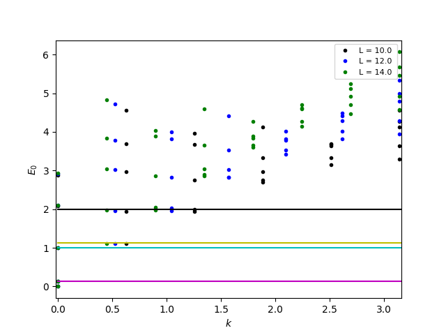
We therefore expect scaling dimensions of 0, 1/8, 1, 1+1/8 to appear in the CFT of the Ising model. To see this, we will rescale all energies of the spectrum according to . This will force the two lowest states to occur where we expect the scaling dimensions; we can then check whether the rest of the spectrum is consistent with this.
Parameters
| Parameter | Meaning | Value |
|---|---|---|
LATTICE | lattice used for the chain | chain lattice |
MODEL | Hamiltonian family | spin |
local_S | spin quantum number per site | 0.5 |
Jxy | in-plane () coupling, unused here | 0 |
Jz | Ising () coupling | -1 |
Gamma | transverse field | 0.5 |
NUMBER_EIGENVALUES | number of low-lying eigenstates kept | 5 |
L | chain length | 10, 12 |
With Jz=-1 and Gamma=0.5, , which is exactly the critical point of the model.
Lattice
The chain lattice is a 1D periodic ring of L sites, with the Ising coupling living on the bonds and the transverse field acting on each site:
 Γ       Γ       Γ             Γ
 o--Jz---o--Jz---o--- ... ---o
 |                            |
 +------------ Jz ------------+
        (periodic ring, L sites)
The ring closes on itself: the bond from the last site back to the first is what makes the lattice periodic. This is the right choice here for two reasons. Periodic boundaries preserve translational symmetry, so each eigenstate carries a well-defined lattice momentum — that is exactly the TOTAL_MOMENTUM quantum number the spectrum is plotted against below. They also have no open ends, so there are no edge states to contaminate the bulk conformal spectrum, and finite-size corrections to the CFT scaling dimensions fall off faster than they would on an open chain. If you want open boundaries instead, ALPS provides open chain lattice; see the ALPS lattice library for the full list of built-in lattices.
Method Choice
The full Hilbert space of the spin-1/2 chain has dimension — for and for . Since only the lowest few eigenstates are needed (not the full spectrum), the iterative Lanczos algorithm implemented by sparsediag is the natural choice: it converges the lowest eigenvalues in far fewer matrix-vector multiplications than a full diagonalization would need, and both Hilbert space sizes here are trivially within its reach (runtime well under a second per system size).
Simulation
We will first import some modules:
import pyalps
import pyalps.plot
import numpy as np
import matplotlib.pyplot as plt
import copy
import math
Then, let us set up the parameters for two system sizes. Be careful to use the transverse field , not the longitudinal field .
# Some general parameters with different lattice sizes:
parms = []
for L in [10,12]:
    parms.append({
        'LATTICE'    : "chain lattice",
        'MODEL'      : "spin",
        'local_S'    : 0.5,
        'Jxy'        : 0,
        'Jz'         : -1,
        'Gamma'      : 0.5,
        'NUMBER_EIGENVALUES' : 5,
        'L'          : L
    })
As you can see, we will simulate two system sizes. Now let’s set up the input files and run the simulation:
prefix = 'ising'
input_file = pyalps.writeInputFiles(prefix,parms)
res = pyalps.runApplication('sparsediag', input_file)
# res = pyalps.runApplication('sparsediag', input_file, MPI=2, mpirun='mpirun')
data = pyalps.loadEigenstateMeasurements(pyalps.getResultFiles(prefix=prefix))
To perform CFT assignments, we need to calculate the ground state and the first excited state for each L. The output of the above load operation will be a hierarchical list sorted by L, so we can just iterate through it
E0 = {}
E1 = {}
for Lsets in data:
    L = pyalps.flatten(Lsets)[0].props['L']
    # Make a big list of all energy values
    allE = []
    for q in pyalps.flatten(Lsets):
        allE += list(q.y)
    allE = np.sort(allE)
    E0[L] = allE[0]
    E1[L] = allE[1]
Subtract E0, divide by gap, multiply by 1/8, which we know to be the smallest non-vanishing scaling dimension of the Ising CFT
for q in pyalps.flatten(data):
    L = q.props['L']
    q.y = (q.y-E0[L])/(E1[L]-E0[L]) * (1./8.)

spectrum = pyalps.collectXY(data, 'TOTAL_MOMENTUM', 'Energy', foreach=['L'])
Plot the first few exactly known scaling dimensions
for SD in [0.125, 1, 1+0.125, 2]:
    d = pyalps.DataSet()
    d.x = np.array([0,4])
    d.y = SD+0*d.x
    # d.props['label'] = str(SD)
    spectrum += [d]

pyalps.plot.plot(spectrum)

plt.legend(prop={'size':8})
plt.xlabel("$k$")
plt.ylabel("$E_0$")

plt.xlim(-0.02, math.pi+0.02)

plt.show()
The result of the simulation is shown in the figure:
Results
Running the code above at the critical point (, ) gives the raw ground- and first-excited-state energies:
| 10 | -3.19623 | -3.15688 | 0.03935 |
| 12 | -3.83065 | -3.79788 | 0.03277 |
After the rescaling , these two states map to scaling dimensions and by construction; the plot shows whether the rest of the low-lying spectrum falls near the predicted values and .
Summary and Outlook
The rescaled excitation spectrum of the finite critical Ising chain reproduces the scaling dimensions predicted by the CFT, confirming the field-theory identification of the lattice model’s low-energy sector.
- What happens to the agreement with the CFT predictions as you increase beyond 12?
- How does the spectrum change if you move away from the critical point ()?
- Can you identify the scaling dimension of the next set of descendants above ?