Spectra of 1D Quantum Systems

In this tutorial we will calculate the energy spectra of the quantum Heisenberg model on various 1D lattices. The main work will be done by the sparsediag application, which implements the Lanczos algorithm, an iterative eigensolver, to obtain energies in different momentum sectors. The collected data will be plotted to show the energy-momentum spectra of 1D quantum Heisenberg model on various 1D lattices.

Heisenberg Chain

Introduction

The Hamiltonian for the spin-1/2 Heisenberg chain, first introduced by W. Heisenberg, Zeitschrift für Physik 49, 619-636 (1928), is given by

H = J\sum_{\langle i,j \rangle} \mathbf{S}^i \cdot \mathbf{S}^j,

where $J>0$ for antiferromagnetic interactions between two nearest-neighbor spins $\mathbf{S}^i$ and $\mathbf{S}^j$ , and the spin-spin interaction consists of three components, i.e.,

\mathbf{S}^i \cdot \mathbf{S}^j=S^i_xS^j_x+S^i_yS^j_y+S^i_zS^j_z.

The basis states are usually chosen to be the eigen states of $S_z$ operator. For a spin-1/2 system, there are two basis states for each lattice site, $|-1/2\rangle$ and $|+1/2\rangle$ . The application of $S_x$ and $S_y$ operators on these basis states can be expressed in terms of raising $S^{\dagger}$ and lowering $S^{-}$ operators:

S_x=\frac{1}{2}(S^{\dagger}+S^{-}),

S_y=\frac{1}{2i}(S^{\dagger}-S^{-}),

who act on the basis states in the following way:

S^{\dagger}|s\rangle = \sqrt{S(S+1)-s(s+1)}|s+1\rangle,

S^{-}|s\rangle = \sqrt{S(S+1)-s(s-1)}|s-1\rangle,

where $S=1/2$ and $s=-1/2, 1/2$ .

With the above basis states for each lattice site, the Hamiltonian can be written as a Hermitian matrix. The size of the matrix can be reduced when the total magnetization is fixed, i.e., setting Sz_total = 0 (singlet sector) or Sz_total = 1 (triplet sector) in the simulations. To further reduce the size of the Hamiltonian matrix and obtain the momentum dependence of the energy spectra, we can further restrict the simulations in different lattice momentum sectors $P=0, 1, 2, \cdots$ .

Parameters: LATTICE="chain lattice", MODEL="spin", local_S=0.5, J=1, CONSERVED_QUANTUMNUMBERS="Sz", Sz_total=0, and L=10,12,14,16.

Lattice:

   J     J     J           J
o-----o-----o-----o-- ... --o     (periodic chain, L sites, coupling J on every bond)

Method choice: the Hilbert space is $2^L$ , e.g. $2^{16}=65536$ at the largest size — small enough for sparsediag’s Lanczos algorithm to find the full low-energy spectrum in every $(S_z, P)$ sector in seconds.

Simulation

To obtain the energy spectrum for the Heisenberg chain, we follow the steps below.

We first import the required modules.

import pyalps
import numpy as np
import matplotlib as plt
import pyalps.plot

Prepare the input parameters for 4 different lattice sizes: $L=10, 12, 14$ , and $16$ .

parms=[]
for l in [10, 12, 14, 16]:
    parms.append(
      { 
        'LATTICE'                   : "chain lattice", 
        'MODEL'                     : "spin",
        'local_S'                   : 0.5,
        'J'                         : 1,
        'L'                         : l,
        'CONSERVED_QUANTUMNUMBERS'  : 'Sz',
        'Sz_total'                  : 0
      }
    )

Write the input file and run the simulation.

input_file = pyalps.writeInputFiles('parm_chain',parms)
res = pyalps.runApplication('sparsediag',input_file)

Load all measurements for all states, and collect spectra over all momenta for every simulation.

data = pyalps.loadSpectra(pyalps.getResultFiles(prefix='parm_chain'))

spectra = {}
for sim in data:
  l = int(sim[0].props['L'])
  all_energies = []
  spectrum = pyalps.DataSet()
  for sec in sim:
    all_energies += list(sec.y)
    spectrum.x = np.concatenate((spectrum.x,np.array([sec.props['TOTAL_MOMENTUM'] for i in range(len(sec.y))])))
    spectrum.y = np.concatenate((spectrum.y,sec.y))
  spectrum.y -= np.min(all_energies)
  spectrum.props['line'] = 'scatter'
  spectrum.props['label'] = 'L='+str(l)
  spectra[l] = spectrum

Plot the energy vs. momentum spectrum.

plt.pyplot.figure()
pyalps.plot.plot(spectra.values())
plt.pyplot.legend()
plt.pyplot.title('Antiferromagnetic Heisenberg chain (S=1/2)')
plt.pyplot.ylabel('Energy')
plt.pyplot.xlabel('Momentum')
plt.pyplot.xlim(0,2*3.1416)
plt.pyplot.ylim(0,2)
plt.pyplot.show()

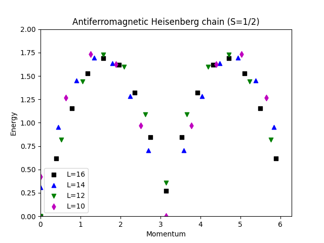
Below is the energy spectrum for a 1D Heisenberg chain: Energy spectrum Heisenberg chain

Two-leg Heisenberg Ladder

Introduction

The Hamiltonian for the two-leg spin-1/2 Heisenberg chain is given by

H = J_0\sum_{\langle \alpha i,\alpha j \rangle} \mathbf{S}^{\alpha i} \cdot \mathbf{S}^{\alpha j} + J_1\sum_{\langle 1 i,2 i \rangle} \mathbf{S}^{1 i} \cdot \mathbf{S}^{2 i},

where, $\alpha=1,2$ denotes the two legs/chains, $i,j=1,2,\cdots,L$ label lattice sites within a chain, $J_0>0$ is the intra-chain antiferromagnetic interactions between two nearest-neighbor spins $\mathbf{S}^{\alpha i}$ and $\mathbf{S}^{\alpha j}$ in the same chain, and $J_1>0$ is the inter-chain spin-spin coupling between $\mathbf{S}^{1 i}$ from the first leg and $\mathbf{S}^{2 i}$ from the second leg with $i=1,2,\cdots,L$ .

Parameters: LATTICE="ladder", MODEL="spin", local_S=0.5, J0=1, J1=1, CONSERVED_QUANTUMNUMBERS="Sz", Sz_total=0, and L=6,8,10.

Lattice:

o--J0--o--J0--o    (leg 1)
|      |      |
J1     J1     J1
|      |      |
o--J0--o--J0--o    (leg 2, L rungs total)

Method choice: the ladder has $2L$ sites, so the Hilbert space is $2^{2L}$ — $2^{20}\approx10^6$ at $L=10$ — still well within reach of sparsediag’s Lanczos solver once the $S_z=0$ restriction is applied.

Simulation

We first import the required modules.

import pyalps
import numpy as np
import matplotlib as plt
import pyalps.plot

Prepare the input parameters by setting values for the intra- and inter-chain interactions J0 and J1, and the chain lengths L=6,8, and 10.

parms=[]
for l in [6, 8, 10]:
    parms.append(
      { 
        'LATTICE'                   : "ladder", 
        'MODEL'                     : "spin",
        'local_S'                   : 0.5,
        'J0'                        : 1,
        'J1'                        : 1,
        'L'                         : l,
        'CONSERVED_QUANTUMNUMBERS'  : 'Sz',
        'Sz_total'                  : 0
      }
    )

Write the input file and run the simulation

input_file = pyalps.writeInputFiles('parm_ladder',parms)
res = pyalps.runApplication('sparsediag',input_file)

Load all measurements for all states, and collect spectra over all momenta for every simulation.

data = pyalps.loadSpectra(pyalps.getResultFiles(prefix='parm_ladder'))

spectra = {}
for sim in data:
  l = int(sim[0].props['L'])
  all_energies = []
  spectrum = pyalps.DataSet()
  for sec in sim:
    all_energies += list(sec.y)
    spectrum.x = np.concatenate((spectrum.x,np.array([sec.props['TOTAL_MOMENTUM'] for i in range(len(sec.y))])))
    spectrum.y = np.concatenate((spectrum.y,sec.y))
  spectrum.y -= np.min(all_energies)
  spectrum.props['line'] = 'scatter'
  spectrum.props['label'] = 'L='+str(l)
  spectra[l] = spectrum

Plot the energy spectrum.

plt.pyplot.figure()
pyalps.plot.plot(spectra.values())
plt.pyplot.legend()
plt.pyplot.title('Antiferromagnetic Heisenberg ladder (S=1/2)')
plt.pyplot.ylabel('Energy')
plt.pyplot.xlabel('Momentum')
plt.pyplot.xlim(0,2*3.1416)
plt.pyplot.ylim(0,2.5)
plt.pyplot.show()

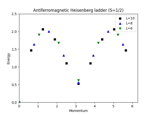
Below shows the energy spectrum for a Heisenberg ladder: Energy spectrum Heisenberg ladder

Isolated Dimers

Introduction

For our third simulation, we start with the same Hamiltonian as in the previous case

H = J_0\sum_{\langle \alpha i,\alpha j \rangle} \mathbf{S}^{\alpha i} \cdot \mathbf{S}^{\alpha j} + J_1\sum_{\langle 1 i,2 i \rangle} \mathbf{S}^{1 i} \cdot \mathbf{S}^{2 i},

where, $\alpha=1,2$ denotes the two legs/chains, $i,j=1,2,\cdots,L$ label lattice sites within a chain, we set $J_0=0$ , i.e., no intra-chain interactions between two nearest-neighbor spins, and $J_1=1$ is the inter-chain spin-spin coupling between $\mathbf{S}^{1 i}$ and $\mathbf{S}^{2 i}$ with $i=1,2,\cdots,L$ . The system then becomes $L$ isolated dimers.

Parameters: same ladder lattice and spin model as above, but with J0=0 (legs decoupled) and J1=1, for L=6,8,10.

Lattice:

o      o      o
|      |      |
J1     J1     J1     (J0 = 0: no leg bonds → L independent dimers)
|      |      |
o      o      o

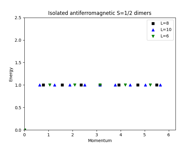
Method choice: setting $J_0=0$ decouples the ladder into $L$ independent 2-site dimers, so the exact spectrum is known analytically (each dimer contributes a singlet at $E=-3J_1/4$ and a triplet at $E=J_1/4$ ); this case is included as a sanity check on the sparsediag results for the coupled ladder above.

Simulation

We first import the required modules.

import pyalps
import numpy as np
import matplotlib as plt
import pyalps.plot

Prepare the input parameters.

parms=[]
for l in [6, 8, 10]:
    parms.append(
      { 
        'LATTICE'                   : "ladder", 
        'MODEL'                     : "spin",
        'local_S'                   : 0.5,
        'J0'                        : 0,
        'J1'                        : 1,
        'L'                         : l,
        'CONSERVED_QUANTUMNUMBERS'  : 'Sz',
        'Sz_total'                  : 0
      }
    )

Write the input file and run the simulation.

input_file = pyalps.writeInputFiles('parm_dimers',parms)
res = pyalps.runApplication('sparsediag',input_file)

Load all measurements for all states.

data = pyalps.loadSpectra(pyalps.getResultFiles(prefix='parm_dimers'))

Collect spectra over all momenta for every simulation.

spectra = {}
for sim in data:
  l = int(sim[0].props['L'])
  all_energies = []
  spectrum = pyalps.DataSet()
  for sec in sim:
    all_energies += list(sec.y)
    spectrum.x = np.concatenate((spectrum.x,np.array([sec.props['TOTAL_MOMENTUM'] for i in range(len(sec.y))])))
    spectrum.y = np.concatenate((spectrum.y,sec.y))
  spectrum.y -= np.min(all_energies)
  spectrum.props['line'] = 'scatter'
  spectrum.props['label'] = 'L='+str(l)
  spectra[l] = spectrum

We then plot the energy spectrum.

plt.pyplot.figure()
pyalps.plot.plot(spectra.values())
plt.pyplot.legend()
plt.pyplot.title('Isolated antiferromagnetic S=1/2 dimers')
plt.pyplot.ylabel('Energy')
plt.pyplot.xlabel('Momentum')
plt.pyplot.xlim(0,2*3.1416)
plt.pyplot.ylim(0,2.5)
plt.pyplot.show()

The energy spectrum for the isolated Heisenberg dimers is shown below: Energy spectrum of isolated Heisenberg dimers

Results

Ground-state energies and the gap to the first excited state, from running the code above:

System	$L$	$E_0$	$E_0/L$	Gap to $E_1$
Chain	10	-4.51545	-0.45154	0.42324
Chain	12	-5.38739	-0.44895	0.35585
Chain	14	-6.26355	-0.44740	0.30711
Chain	16	-7.14230	-0.44639	0.27019
Ladder	6	-7.01325	-0.58444	0.62657
Ladder	8	-9.28325	-0.58020	0.55740
Ladder	10	-11.57719	-0.57772	0.52811
Dimers	6	-4.50000	-0.75000	1.00000
Dimers	8	-6.00000	-0.75000	1.00000
Dimers	10	-7.50000	-0.75000	1.00000

The chain’s $E_0/L$ is trending toward the exact thermodynamic-limit value $-\ln2+1/4\approx-0.4431$ as $L$ grows, and the isolated-dimer case reproduces the exact analytic result $E_0/L=-3J_1/4=-0.75$ and gap $=J_1=1$ to machine precision — a useful check that the ladder result in between ( $J_0=J_1=1$ ) is trustworthy.

Summary and Outlook

Exact diagonalization on finite 1D lattices reproduces the expected gapless spectrum of the Heisenberg chain, the larger spin gap of the two-leg ladder (a consequence of the extra inter-chain coupling), and the exactly solvable isolated-dimer limit used here as a benchmark.

As $J_1/J_0$ is increased from the isolated-chain limit, at what point does the ladder’s gap approach the isolated-dimer value $J_1$ ?
How would you expect the momentum-resolved spectrum to change for a three-leg ladder?
Can you verify the isolated-dimer results analytically from the two-site Heisenberg Hamiltonian?

Spin Gap of a Spin-1 Heisenberg Chain Ground State Energy of a Spin Chain