Spin Gap of a Spin-1 Heisenberg Chain
In this tutorial we will learn how to use the sparse diagonalization program (Lanczos algorithm) to calculate the energy gaps of a 1D spin-1 Heisenberg chain for various lattice sizes (, and 10). The obtained finite-lattice gaps are then used to extrapolate the energy gap in the thermodynamic limit ().
The Hamiltonian for the spin-1 Heisenberg chain is given by
where for antiferromagnetic interactions between two nearest-neighbor spins and , and the spin-spin interaction consists of three components, i.e.,
The basis states are usually chosen to be the eigen states of operator. For a spin-1 system, there are three basis states for each lattice site, , , and . The application of and operators on these basis states can be expressed in terms of raising and lowering operators:
who act on the basis states in the following way:
where and .
With the above basis states for each lattice site, the Hamiltonian can be written as a Hermitian matrix. The size of the matrix can be reduced when the total magnetization is fixed, i.e., setting Sz_total = 0 (singlet sector) or Sz_total = 1 (triplet sector) in the simulations.
The Heisenberg exchange Hamiltonian was introduced by W. Heisenberg, Zeitschrift für Physik 49, 619-636 (1928). For an integer-spin chain (such as here), F.D.M. Haldane, Physics Letters A 93, 464-468 (1983) predicted — contrary to the gapless spin-1/2 case — a finite excitation gap in the thermodynamic limit, now known as the Haldane gap.
Parameters
| Parameter | Meaning | Value |
|---|---|---|
LATTICE | lattice used for the chain | chain lattice |
MODEL | Hamiltonian family | spin |
local_S | spin quantum number per site | 1 |
J | Heisenberg exchange coupling | 1 |
L | chain length | 4, 6, 8, 10, 12, 14 |
CONSERVED_QUANTUMNUMBERS | quantum numbers fixed in the basis | Sz |
Sz_total | total magnetization sector | 0 (singlet), 1 (triplet) |
Lattice
The chain lattice is a 1D periodic ring of L spin-1 sites coupled by nearest-neighbour exchange :
 S=1     S=1     S=1           S=1
  o---J---o---J---o--- ... ---o
  |                           |
  +----------- J -------------+
        (periodic ring, L sites)
The bond from the last site back to the first closes the ring. Periodic boundaries matter for this particular calculation: an open spin-1 chain carries effective spins localized at its two ends, and the near-degenerate edge states they produce sit inside the bulk gap, so the measured singlet/triplet splitting on an open chain is an edge excitation rather than the Haldane gap. Closing the chain into a ring removes the ends entirely, so the gap extracted below is the bulk gap that the extrapolation is after. See the ALPS lattice library for other built-in lattices, including open chain lattice.
Method Choice
For spin-1, the local Hilbert space has dimension 3, so the full Hilbert space of an -site chain is — e.g. before the Sz_total restriction cuts it down substantially. Since only the lowest energy in each Sz_total sector is needed, the Lanczos-based sparsediag is again the appropriate method rather than a full diagonalization: all six lattice sizes used here ( to ) complete in well under a minute in total.
We first import the required modules.
import pyalps
import numpy as np
import matplotlib.pyplot as plt
import pyalps.plot
import pyalps.fit_wrapper as fw
Then we prepare the input files as a list of Python dictionaries.
parms = []
for l in [4, 6, 8, 10, 12, 14]:
  for sz in [0, 1]:
      parms.append(
        {
          'LATTICE'                   : "chain lattice",
          'MODEL'                     : "spin",
          'local_S'                   : 1,
          'J'                         : 1,
          'L'                         : l,
          'CONSERVED_QUANTUMNUMBERS'  : 'Sz',
          'Sz_total'                  : sz
        }
      )
We write the input file and run the simulation.
input_file = pyalps.writeInputFiles('parm2a',parms)
res = pyalps.runApplication('sparsediag',input_file) #, MPI=4)
We next load the spectra for each of the systems sizes and spin sectors:
data = pyalps.loadSpectra(pyalps.getResultFiles(prefix='parm2a'))To extract the gaps we need to write a few lines of Python, to set up a list of lengths and a Python dictionaries of the minimum energy in each (L,Sz) sector:
lengths = []
min_energies = {}

for sim in data:
  l = int(sim[0].props['L'])
  if l not in lengths: lengths.append(l)
  sz = int(sim[0].props['Sz_total'])
  all_energies = []
  for sec in sim:
    all_energies += list(sec.y)
  min_energies[(l,sz)]= np.min(all_energies)
And finally we make a plot of the gap as a function of 1/L and then show the plot
gapplot = pyalps.DataSet()
gapplot.x = 1./np.sort(lengths)
gapplot.y = [min_energies[(l,1)] -min_energies[(l,0)] for l in np.sort(lengths)]
gapplot.props['xlabel']='$1/L$'
gapplot.props['ylabel']='Triplet gap (J)'
gapplot.props['label']='S=1'
gapplot.props['line']='.'

plt.figure()
pyalps.plot.plot(gapplot)
plt.legend()
plt.xlim(0,0.25)
plt.ylim(0,1.0)
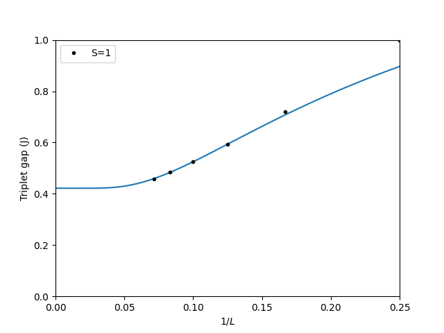
We then fit the data in the range L=8 to L=14 to obtain the gap in the thermodynamic limit ( or ).
pars = [fw.Parameter(0.411), fw.Parameter(1000), fw.Parameter(1)]
f = lambda self, x, p: p[0]()+p[1]()*np.exp(-x/p[2]())
fw.fit(None, f, pars, np.array(gapplot.y)[2:], np.sort(lengths)[2:])

x = np.linspace(0.0001, 1./min(lengths), 100)
plt.plot(x, f(None, 1/x, pars))

plt.show()
The result of the simulation is shown in the figure:
Results
Running the code above gives the following finite-size triplet gaps and extrapolated value:
| Gap | |
|---|---|
| 4 | 1.00000 |
| 6 | 0.72063 |
| 8 | 0.59356 |
| 10 | 0.52481 |
| 12 | 0.48420 |
| 14 | 0.45897 |
Fitting to to extrapolates to , close to the numerically-known Haldane gap value (the ~3% deviation is finite-size fitting error, since only is used here).
Summary and Outlook
Exact diagonalization of finite spin-1 Heisenberg chains, extrapolated to , confirms the finite Haldane gap predicted for integer-spin antiferromagnetic chains — in sharp contrast to the gapless spin-1/2 chain.
- How does the extrapolated gap change if you include larger in the fit, or use only the largest three sizes?
- What functional form would you expect for the gap in a spin-1/2 chain, where no gap is present?
- How sensitive is the extrapolated to the choice of fit range?