MC-01a Autocorrelations

In Monte Carlo simulations of this type, consecutive samples are not statistically independent: each configuration is generated from the previous one, so the data are correlated in time. The autocorrelation time $\tau$ measures how many MC sweeps must separate two samples before they can be treated as independent. If $\tau$ is large compared to the total number of sweeps, naive error estimates — which assume independent samples — will be too small and the results untrustworthy. This problem is most severe near a phase transition, where the correlation length diverges and local updates become very inefficient.

This tutorial demonstrates the issue using the 2D Ising model at its critical temperature and shows how switching from local (Metropolis) updates to cluster updates dramatically reduces autocorrelation times. The key diagnostic tool is a binning analysis: errors are recomputed after grouping samples into successively larger bins; if the estimated error has not plateaued by the largest bin size, the autocorrelation time is longer than the run and the errors cannot be trusted.

The input files for this tutorial are available in your ALPS distribution in the directory mc-01-autocorrelations.

Local updates

We will simulate an Ising model on finite square lattices (L=2, 4, …, 48) at the critical temperature $T_C=2.269186$ using local updates. This tutorial can be run either on the command line or in Python. We recommend the Python version on your local machine, and the command line version for large simulations on clusters.

Setting up and running the simulation on the command line

To set up and run the simulation on the command line, we first create a parameter file that specifies the parameters of the simulation(s). The downloadable file will be titled parm1a, with the following contents:

LATTICE="square lattice"
T=2.269186
J=1
THERMALIZATION=10000
SWEEPS=50000  
UPDATE="local"
MODEL="Ising"
{L=2;}
{L=4;}
{L=8;}
{L=16;}
{L=32;}
{L=48;}

This actually specifies six simulation tasks in one simulation job, all tasks having identical parameters except for the lattice length L.

ALPS expects one job file to specify the job as a whole and a task file for each simulation task within it, all in XML format. So in order to run the simulation, we first need to convert this parameter file. ALPS provides a simple tool to do this: We can just run

parameter2xml parm1a

in the folder of the parameter file. This will generate six task files (one for each length L) named parm1a.task1.in.xml through parm1a.task6.in.xml and a job description file parm1a.in.xml. We can open the job file with an XML browser to check the status of our simulation once we have started it.

The simulation can be started on a single processor by running

spinmc --Tmin 10 --write-xml parm1a.in.xml

or on multiple processors (eight in this example) using MPI:

mpirun -np 8 spinmc --mpi  --Tmin 10 --write-xml parm1a.in.xml

(In the following examples we will refer to the single-processor commands only.) By setting the argument --Tmin 10, we tell the scheduler to check if the simulation is finished every 10 seconds initially. (The time is then dynamically adapted by the scheduler according to the needs of the simulation.)

The progress of a simulation is saved in the XML output file as the simulation is run. If a simulation is halted, for example by pressing Ctrl-C or reaching the CPU time limit, it may be continued by starting the simulation with the XML output file instead of the input job file. Since our input job file was named parm1a.in.xml, the output file will be named parm1a.out.xml and we may restart the simulation by running

spinmc --Tmin 10 --write-xml parm1a.out.xml

The option “–write-xml” tells the simulation to store the results of each simulation also in an XML output file (parm1a.task\[1-6\].out.xml) which you can open from the job description file parm1a.out.xml using your XML browser or alternatively by converting the output to a text file using one of the following commands:

firefox ./parm1a.out.xml
convert2text parm1a.out.xml

The results of a single task stored, for example, in parm1a.task1.out.xml, can be displayed by using either of the following commands:

Linux: firefox ./parm1a.task1.out.xml
MacOS: open -a safari parm1a.task1.out.xml
Text output: convert2text parm1a.task1.out.xml

Note that writing XML files can be very slow if you perform many measurements, and it is then better to work with the binary results in the HDF5 files.

To obtain more detailed information on the simulation runs, such as to check the convergence of errors, we can convert the run files of the tasks (parm1a.task\[1-6\].out.run1) into XML files by typing

convert2xml parm1a.task*.out.run1

which will generate the XML output files parm1a.task\[1-6\].out.run1.xml, which can be opened or converted to text just like the output XML files.

Look at all six tasks and, by studying the binning analysis in the files parm1a.task\[1-6\].out.run1.xml, observe that for large lattices the errors no longer converge. To create plots, we recommend using the Python tools described below.

Setting up and running the simulation in Python

The pyalps package is a wrapper for ALPS: All it does is call the commands described in the previous section as if they were run in a terminal. It is superior for plotting because the output of the simulation can be read directly into a Python data structure and accessed by matplotlib, and it also comes with a wrapper pyalps.plot for certain matplotlib functions to neatly plot data generated by pyalps.

To set up and run the simulation in Python, we create a script named tutorial1a.py. The first part of this script must import the required modules and prepare the input job and task files. Instead of writing a parameter file and using convert2xml, we store a list containing each task’s parameters as a dictionary, like so:

import pyalps
import matplotlib.pyplot as plt
import pyalps.plot

parms = []
for l in [2,4,8,16,32,48]:
    parms.append(
        {
            'LATTICE'        : "square lattice",
            'T'              : 2.269186,
            'J'              : 1 ,
            'THERMALIZATION' : 10000,
            'SWEEPS'         : 50000,
            'UPDATE'         : "local",
            'MODEL'          : "Ising",
            'L'              : l
        }
    )

and convert this into an XML job file with the function

input_file = pyalps.writeInputFiles('parm1a',parms)

The input_file variable may be used as an input for pyalps.runApplication as shown below:

pyalps.runApplication('spinmc',input_file,Tmin=5,writexml=True)

spinmc is the name of the terminal command to be called. The option writexml=True tells ALPS to write XML files, input_file is the path to the XML job input file, and Tmin=5 again tells ALPS to check every 5 seconds for completion of the simulation.

We next load the binning analysis for the absolute value of the magnetization from the output files using pyalps.loadBinningAnalysis, and flatten the list of lists we get with pyalps.flatten:

binning = pyalps.loadBinningAnalysis(pyalps.getResultFiles(prefix='parm1a'),'|Magnetization|')
binning = pyalps.flatten(binning)

We give each dataset a label that will appear in the plot legend to identify the lattice size:

for dataset in binning:
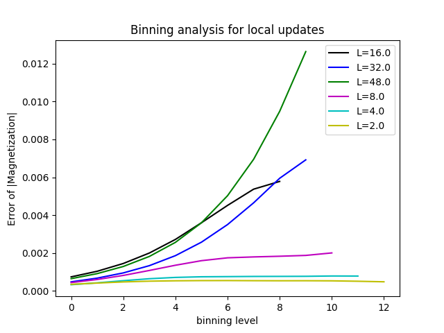
    dataset.props['label'] = 'L='+str(dataset.props['L'])

pyalps.plot functions will use these labels automatically. Finally, we create a plot showing the binning analysis:

plt.figure()
plt.xlabel('binning level')
plt.ylabel('Error of |Magnetization|')
pyalps.plot.plot(binning)
plt.legend()
plt.show()

To make separate plots for each system size we make a loop over all data sets:

for dataset in binning:
    plt.figure()
    plt.title('Binning analysis for L='+str(dataset.props['L']))
    plt.xlabel('binning level')
    plt.ylabel('Error of |Magnetization|')
    pyalps.plot.plot(dataset)
    
plt.show()

From the figure below, you can clearly see that the errors do not converge for large system sizes.

Cluster updates

Near the critical temperature, the correlation length $\xi$ grows large and local updates become highly inefficient: each accepted move flips a single spin, so it takes $O(\xi^2)$ sweeps merely to decorrelate two neighbouring spins. This critical slowing down means the autocorrelation time diverges as $$\tau \sim L^z,$$ where $z \approx 2$ for local updates but $z \approx 0.25$ for cluster algorithms such as Wolff or Swendsen–Wang. Cluster updates flip entire correlated regions at once, essentially eliminating critical slowing down for the quantities measured here.

We therefore repeat the simulations with cluster updates, using fewer thermalization sweeps (the system decorrelates much faster) but more measurement sweeps to accumulate good statistics:

Parameter	Value
THERMALIZATION	1000
SWEEPS	100000
UPDATE	“cluster”

Command line

The downloadable parameter file parm1b has the following contents:

LATTICE="square lattice"
T=2.269186
J=1
THERMALIZATION=1000
SWEEPS=100000
UPDATE="cluster"
MODEL="Ising"
{L=2;}
{L=4;}
{L=8;}
{L=16;}
{L=32;}
{L=48;}

Convert and run exactly as before:

parameter2xml parm1b
spinmc --Tmin 10 --write-xml parm1b.in.xml

Python

The script tutorial1b.py follows the same structure as tutorial1a.py, with the updated parameters and parm1b as the file prefix:

import pyalps
import matplotlib.pyplot as plt
import pyalps.plot

parms = []
for l in [2,4,8,16,32,48]:
    parms.append(
        {
            'LATTICE'        : "square lattice",
            'T'              : 2.269186,
            'J'              : 1,
            'THERMALIZATION' : 1000,
            'SWEEPS'         : 100000,
            'UPDATE'         : "cluster",
            'MODEL'          : "Ising",
            'L'              : l
        }
    )

input_file = pyalps.writeInputFiles('parm1b', parms)
pyalps.runApplication('spinmc', input_file, Tmin=5, writexml=True)

binning = pyalps.loadBinningAnalysis(pyalps.getResultFiles(prefix='parm1b'), '|Magnetization|')
binning = pyalps.flatten(binning)

for dataset in binning:
    dataset.props['label'] = 'L=' + str(dataset.props['L'])

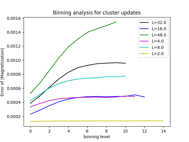
plt.figure()
plt.xlabel('binning level')
plt.ylabel('Error of |Magnetization|')
pyalps.plot.plot(binning)
plt.legend()
plt.show()

You will get curves looking like the ones below. Now the errors have converged and can be trusted.

Questions

Are the errors converged? (To check this convert the run files as described above.)
Why do longer autocorrelation times lead to slower error convergence?
On what system parameters do the autocorrelation times depend? Check by changing parameters in the input file.
Can you explain why cluster updates are more efficient than local updates?

Which code to choose for your calculation MC-01b Equilibration