MC-02 Susceptibilities
The magnetic susceptibility measures how strongly a system responds to a small applied magnetic field. Its temperature dependence is a sensitive probe of the underlying spin correlations: a system of weakly interacting spins follows the Curie law , while interactions and quantum effects produce characteristic deviations.
This tutorial calculates for four systems — classical and quantum Heisenberg models on one-dimensional chains and two-leg ladders — and overlays the results on a single plot. The comparison highlights two key contrasts: how quantum fluctuations modify the classical picture, and how changing the lattice geometry from a chain to a ladder affects the low-temperature behaviour.
Sign convention. The classical
spinmccode and the quantumloopercode both use the Hamiltonian , where favours ferromagnetic alignment and favours antiferromagnetic alignment. The classical simulations below use (ferromagnet); the quantum simulations use (antiferromagnet). Both choices produce a positive susceptibility that grows at low temperature, making the comparison of classical versus quantum behaviour straightforward.
Classical Heisenberg models
One-dimensional chain
Setting up and running on the command line
The parameter file parm2a sets up simulations of the classical ferromagnetic Heisenberg model on a chain of 60 sites across a range of temperatures:
LATTICE="chain lattice"
L=60
J=-1
THERMALIZATION=15000
SWEEPS=500000
UPDATE="cluster"
MODEL="Heisenberg"
{T=0.05;}
{T=0.1;}
{T=0.2;}
{T=0.3;}
{T=0.4;}
{T=0.5;}
{T=0.6;}
{T=0.7;}
{T=0.8;}
{T=0.9;}
{T=1.0;}
{T=1.25;}
{T=1.5;}
{T=1.75;}
{T=2.0;}
Run the simulation with the standard sequence:
parameter2xml parm2a
spinmc --Tmin 10 --write-xml parm2a.in.xml
Setting up and running in Python
The script tutorial2a.py sets up and runs the same simulation. Place it in the same folder as parm2a:
import pyalps
import matplotlib.pyplot as plt
import pyalps.plot

parms = []
for t in [0.05, 0.1, 0.2, 0.3, 0.4, 0.5, 0.6, 0.7, 0.8, 0.9, 1.0, 1.25, 1.5, 1.75, 2.0]:
    parms.append(
        {
            'LATTICE'        : "chain lattice",
            'T'              : t,
            'J'              : -1,
            'THERMALIZATION' : 10000,
            'SWEEPS'         : 500000,
            'UPDATE'         : "cluster",
            'MODEL'          : "Heisenberg",
            'L'              : 60
        }
    )

input_file = pyalps.writeInputFiles('parm2a', parms)
pyalps.runApplication('spinmc', input_file, Tmin=5, writexml=True)
Evaluating and plotting
Load the susceptibility from the output files and plot it against temperature:
import pyalps
import matplotlib.pyplot as plt
import pyalps.plot

data = pyalps.loadMeasurements(pyalps.getResultFiles(prefix='parm2a'), 'Susceptibility')
susceptibility = pyalps.collectXY(data, x='T', y='Susceptibility')

plt.figure()
pyalps.plot.plot(susceptibility)
plt.xlabel('Temperature $T/J$')
plt.ylabel('Susceptibility $\chi J$')
plt.ylim(0, 0.22)
plt.title('Classical Heisenberg chain')
plt.show()
Two-leg ladder
The ladder geometry introduces a second coupling along the rungs in addition to the leg coupling . Aside from the lattice change and the two couplings, the simulation setup is identical to the chain case.
Setting up and running on the command line
Download parm2b and place it in the same folder:
LATTICE="ladder"
L=60
J0=-1
J1=-1
THERMALIZATION=15000
SWEEPS=500000
UPDATE="cluster"
MODEL="Heisenberg"
{T=0.05;}
{T=0.1;}
{T=0.2;}
{T=0.3;}
{T=0.4;}
{T=0.5;}
{T=0.6;}
{T=0.7;}
{T=0.8;}
{T=0.9;}
{T=1.0;}
{T=1.25;}
{T=1.5;}
{T=1.75;}
{T=2.0;}
Run the simulation:
parameter2xml parm2b
spinmc --Tmin 10 --write-xml parm2b.in.xml
Setting up and running in Python
The script tutorial2b.py is a copy of tutorial2a.py with three changes: the prefix renamed to parm2b, LATTICE set to "ladder", and J replaced by J0 and J1 (both -1).
Quantum Heisenberg models
The quantum simulations use the ALPS model library to specify an quantum spin model and the looper QMC code to run the simulations.
The key parameter changes from the classical case are:
MODEL="spin"withlocal_S=1/2instead ofMODEL="Heisenberg"ALGORITHM="loop"to select the looper codeJ=+1for the antiferromagnetic coupling (see sign convention note above)
One-dimensional chain
Setting up and running on the command line
Download parm2c:
LATTICE="chain lattice"
MODEL="spin"
local_S=1/2
L=60
J=1
THERMALIZATION=5000
SWEEPS=50000
ALGORITHM="loop"
{T=0.05;}
{T=0.1;}
{T=0.2;}
{T=0.3;}
{T=0.4;}
{T=0.5;}
{T=0.6;}
{T=0.7;}
{T=0.75;}
{T=0.8;}
{T=0.9;}
{T=1.0;}
{T=1.25;}
{T=1.5;}
{T=1.75;}
{T=2.0;}
Convert and run using the loop application instead of spinmc:
parameter2xml parm2c
loop parm2c.in.xml
Setting up and running in Python
The script tutorial2c.py adapts tutorial2a.py to the quantum parameters and calls loop instead of spinmc:
input_file = pyalps.writeInputFiles('parm2c', parms)
pyalps.runApplication('loop', input_file)
Two-leg ladder
The quantum ladder adds a second coupling J1 along the rungs.
Unlike the gapless chain, the two-leg antiferromagnetic Heisenberg ladder has a spin gap: its ground state is a product of rung singlets, and is exponentially suppressed below the gap energy, falling steeply towards zero at low temperature.
Setting up and running on the command line
Download parm2d:
LATTICE="ladder"
MODEL="spin"
local_S=1/2
L=60
J0=1
J1=1
THERMALIZATION=5000
SWEEPS=50000
ALGORITHM="loop"
{T=0.1;}
{T=0.2;}
{T=0.3;}
{T=0.4;}
{T=0.5;}
{T=0.6;}
{T=0.7;}
{T=0.8;}
{T=1.0;}
{T=1.25;}
{T=1.5;}
{T=1.75;}
{T=2.0;}
parameter2xml parm2d
loop parm2d.in.xmlSetting up and running in Python
The script tutorial2d.py adapts tutorial2c.py: rename the prefix to parm2d, change LATTICE to "ladder", and replace J with J0 and J1 (both 1).
Combining all four simulations
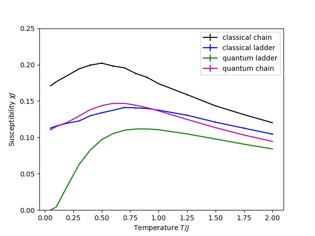
After running all four simulations in the same folder, the script tutorial2full.py loads all results together and overlays them on a single plot.
import pyalps
import matplotlib.pyplot as plt
import pyalps.plot

data = pyalps.loadMeasurements(pyalps.getResultFiles(), 'Susceptibility')
data = pyalps.flatten(data)
pyalps.getResultFiles() with no arguments finds all output files in the current folder; pyalps.flatten merges results from separate files into one list while preserving the simulation parameters for each data point.
We use pyalps.collectXY with the foreach parameter to create a separate curve for each combination of MODEL and LATTICE:
susceptibility = pyalps.collectXY(data, x='T', y='Susceptibility', foreach=['MODEL', 'LATTICE'])Label each curve using its stored parameters:
for s in susceptibility:
    if s.props['LATTICE'] == 'chain lattice':
        s.props['label'] = "chain"
    elif s.props['LATTICE'] == 'ladder':
        s.props['label'] = "ladder"
    if s.props['MODEL'] == 'spin':
        s.props['label'] = "quantum " + s.props['label']
    elif s.props['MODEL'] == 'Heisenberg':
        s.props['label'] = "classical " + s.props['label']
Plot all four curves:
plt.figure()
pyalps.plot.plot(susceptibility)
plt.xlabel('Temperature $T/J$')
plt.ylabel('Susceptibility $\chi J$')
plt.ylim(0, 0.25)
plt.legend()
plt.show()
The resulting plot should look like the figure below. At high temperature all four curves approach the Curie law . At low temperature the quantum ladder drops steeply due to its spin gap, while the classical and quantum chains, and the classical ladder, remain finite or increase.
Questions
- At high temperature, do all four curves approach the same Curie behaviour? What sets the prefactor?
- What is the most visible difference between the classical chain and the quantum chain at low temperature?
- The quantum ladder susceptibility falls much faster than the classical ladder at low . What physical mechanism causes this?
- Try larger system sizes or different lattices (
"cubic lattice","triangular lattice"— seelattices.xml). How do the results change?