MC-03 Magnetization

This tutorial studies magnetization curves $m(h)$ of the $S = 1/2$ Heisenberg model on two geometries: a one-dimensional chain and a two-leg ladder. Because the looper QMC code does not perform well in a magnetic field, we use the directed-loop SSE application dirloop_sse instead.

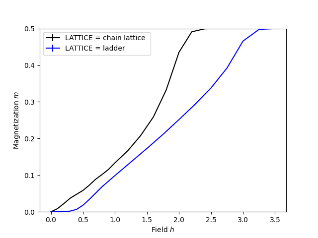
The two geometries produce qualitatively different magnetization curves. The Heisenberg chain is gapless: its magnetization rises smoothly from $m = 0$ as soon as a field is applied. The two-leg ladder has a spin gap $\Delta \approx 0.5J$: the magnetization stays exactly zero for $h < \Delta$ and only begins to rise at a finite critical field, giving a distinctive plateau at $m = 0$.

One-dimensional Heisenberg chain

We simulate the $S = 1/2$ antiferromagnetic Heisenberg chain with 20 sites at temperature $T = 0.08$ across a range of magnetic fields $h = 0, 0.1, \ldots, 2.5$. The temperature is low enough that the results are close to the ground-state magnetization curve.

Setting up and running on the command line

The parameter file parm3a:

LATTICE="chain lattice"
MODEL="spin"
local_S=1/2
L=20
J=1
T=0.08
THERMALIZATION=2000
SWEEPS=10000
{h=0;}
{h=0.1;}
{h=0.2;}
{h=0.3;}
{h=0.4;}
{h=0.5;}
{h=0.6;}
{h=0.7;}
{h=0.8;}
{h=0.9;}
{h=1.0;}
{h=1.2;}
{h=1.4;}
{h=1.6;}
{h=1.8;}
{h=2.0;}
{h=2.2;}
{h=2.4;}
{h=2.5;}

Convert and run using the SSE code:

parameter2xml parm3a
dirloop_sse --Tmin 10 --write-xml parm3a.in.xml

Setting up and running in Python

The script tutorial3a.py:

import pyalps
import matplotlib.pyplot as plt
import pyalps.plot

parms = []
for h in [0., 0.1, 0.2, 0.3, 0.4, 0.5, 0.6, 0.7, 0.8, 0.9, 1.0, 1.2, 1.4, 1.6, 1.8, 2.0, 2.2, 2.4, 2.5]:
    parms.append(
        {
            'LATTICE'        : "chain lattice",
            'MODEL'          : "spin",
            'local_S'        : 0.5,
            'T'              : 0.08,
            'J'              : 1,
            'THERMALIZATION' : 1000,
            'SWEEPS'         : 20000,
            'L'              : 20,
            'h'              : h
        }
    )

input_file = pyalps.writeInputFiles('parm3a', parms)
pyalps.runApplication('dirloop_sse', input_file, Tmin=5)

Evaluating and plotting

Load the magnetization density and plot it as a function of field:

data = pyalps.loadMeasurements(pyalps.getResultFiles(prefix='parm3a'), 'Magnetization Density')
magnetization = pyalps.collectXY(data, x='h', y='Magnetization Density')

plt.figure()
pyalps.plot.plot(magnetization)
plt.xlabel('Field $h/J$')
plt.ylabel('Magnetization $m$')
plt.ylim(0.0, 0.55)
plt.title('Quantum Heisenberg chain')
plt.show()

The magnetization rises continuously from zero, reaching saturation $m = 1/2$ at the saturation field $h_\text{sat} = 2J$.

One-dimensional Heisenberg ladder

The two-leg ladder adds rung couplings $J_1$ connecting the two chains. We use 20 rungs (40 sites total) and extend the field range to $h = 3.5$ to reach saturation.

Setting up and running on the command line

The parameter file parm3b uses the same structure as parm3a with these changes:

LATTICE="ladder"
MODEL="spin"
local_S=1/2
L=20
J0=1
J1=1
T=0.08
THERMALIZATION=2000
SWEEPS=10000
{h=0;}
{h=0.2;}
{h=0.4;}
{h=0.6;}
{h=0.8;}
{h=1.0;}
{h=1.2;}
{h=1.4;}
{h=1.6;}
{h=1.8;}
{h=2.0;}
{h=2.2;}
{h=2.4;}
{h=2.6;}
{h=2.8;}
{h=3.0;}
{h=3.2;}
{h=3.4;}
{h=3.5;}

parameter2xml parm3b
dirloop_sse --Tmin 10 --write-xml parm3b.in.xml

Setting up and running in Python

The script tutorial3b.py adapts tutorial3a.py: rename the prefix to parm3b, change LATTICE to "ladder", replace J with J0=J1=1, and extend the field scan to 3.5.

Evaluating and plotting

data = pyalps.loadMeasurements(pyalps.getResultFiles(prefix='parm3b'), 'Magnetization Density')
magnetization = pyalps.collectXY(data, x='h', y='Magnetization Density')

plt.figure()
pyalps.plot.plot(magnetization)
plt.xlabel('Field $h/J$')
plt.ylabel('Magnetization $m$')
plt.ylim(0.0, 0.55)
plt.title('Quantum Heisenberg ladder')
plt.show()

In contrast to the chain, the ladder magnetization is zero up to a finite lower critical field $h_{c1} \approx \Delta \approx 0.5J$, reflecting the spin gap, before rising to saturation at $h_{c2}$.

Combining both simulations

After running both simulations in the same folder, the script tutorial3full.py overlays the two magnetization curves on a single plot:

import pyalps
import matplotlib.pyplot as plt
import pyalps.plot

data = pyalps.loadMeasurements(pyalps.getResultFiles(), 'Magnetization Density')
magnetization = pyalps.collectXY(data, x='h', y='Magnetization Density', foreach=['LATTICE'])

for m in magnetization:
    if m.props['LATTICE'] == 'chain lattice':
        m.props['label'] = 'chain'
    elif m.props['LATTICE'] == 'ladder':
        m.props['label'] = 'ladder'

plt.figure()
pyalps.plot.plot(magnetization)
plt.xlabel('Field $h/J$')
plt.ylabel('Magnetization $m$')
plt.ylim(0.0, 0.55)
plt.legend()
plt.title('Quantum Heisenberg models')
plt.show()

The combined plot makes the contrast between the gapless chain and the gapped ladder immediately visible.

Questions

At what field does the chain magnetization begin to rise? What does this tell you about the spin gap of the chain?
Estimate the lower critical field $h_{c1}$ of the ladder from your data. How does it compare with the known spin gap $\Delta \approx 0.5J$?
Both models saturate at $m = 1/2$. At what field does saturation occur in each case, and why are the saturation fields different?
Repeat the simulation at a higher temperature, e.g. $T = 0.5$. How do thermal fluctuations affect the sharpness of the features in the magnetization curve?
(Bonus) Try a 3-leg or 4-leg ladder by adding a W parameter for the width, or change local_S to study spin-1 or spin-3/2 chains. Is there a systematic pattern in the critical fields?

MC-02 Susceptibilities MC-04 Measurements