DMFT of Hubbard Model on a Bethe Lattice

The dynamical mean-field theory (DMFT) for strongly correlated electron systems is based on mapping of lattice models onto quantum impurity models subject to a self-consistency condition [Georges, et al, Rev. Mod. Phys. 68, 13 (1996)]. The mapping is exact for models of correlated electrons in the limit of large lattice coordination or infinite spatial dimensions. Bethe lattice is an example lattice with infinite spatial dimensions and can be simulated by DMFT with ALPS.

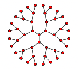
Bethe Lattice

An example picture of Bethe lattice is shown below, where there are 3 coordination numbers for each lattice site. The effective dimension of the lattice is infinite. It, therefore, offers a great opportunity to implement DMFT on such a lattice, where the DMFT method can be benchmarked and explored.

Hubbard Model

We will simulate Hubbard model defined on a Bethe lattice with DMFT. The Hubbard model is defined below. $$ H = -t \sum_{\langle i,j \rangle, \sigma} \left( c_{i,\sigma}^\dagger c_{j,\sigma} + \text{h.c.} \right) + U \sum_i n_{i,\uparrow} n_{i,\downarrow}, $$

where

• $c_{i,\sigma}^\dagger$ and $c_{i,\sigma}$ are creation and annihilation operators for a fermion with flavor $\sigma$ (up $\uparrow$ or down $\downarrow$) at site $i$ and $\text{h.c.}$ represents Hermitian Conjugate.
• $t$ is hopping amplitude between neighboring sites $\langle i,j \rangle$.
• $U$ is on-site interaction energy, with $U > 0$ corresponding to repulsive interactions.
• $n_{i,\sigma} = c_{i,\sigma}^\dagger c_{i,\sigma}$ is number operator for fermions with flavor $\sigma$ at site $i$.

Simulation

We first import the required modules.

import pyalps
import numpy as np
import matplotlib.pyplot as plt
import pyalps.plot

Then we prepare the input files as a list of Python dictionaries.

parms=[]
for b in [6., 12.]: 
    parms.append(
            {                         
              'ANTIFERROMAGNET'         : 1,
              'CONVERGED'               : 0.005,
              'FLAVORS'                 : 2,
              'H'                       : 0,
              'H_INIT'                  : 0.05,
              'MAX_IT'                  : 10,
              'MAX_TIME'                : 10,
              'MU'                      : 0,
              'N'                       : 500,
              'NMATSUBARA'              : 500, 
              'OMEGA_LOOP'              : 1,
              'SEED'                    : 0, 
              'SITES'                   : 1,
              'SOLVER'                  : 'Interaction Expansion',
              'SYMMETRIZATION'          : 0,
              'U'                       : 3,
              't'                       : 0.707106781186547,
              'SWEEPS'                  : 100000000,
              'THERMALIZATION'          : 1000,
              'ALPHA'                   : -0.01,
              'HISTOGRAM_MEASUREMENT'   : 1,
              'BETA'                    : b
            }
        )

The parameter “BETA” refers to inverse temperature and we are simulating the system at two different temperatures, “BETA = 6” at high temperature and “BETA = 12” at low temperature. We then write the input file and run the simulation.

for p in parms:
    input_file = pyalps.writeParameterFile('parm_beta_'+str(p['BETA']),p)
    res = pyalps.runDMFT(input_file)

We next load the result of the simulation.

listobs=['0', '1']
    
data = pyalps.loadMeasurements(pyalps.getResultFiles(pattern='parm_beta_*h5'), respath='/simulation/results/G_tau', what=listobs)
for d in pyalps.flatten(data):
    d.x = d.x*d.props["BETA"]/float(d.props["N"])
    d.props['label'] = r'$\beta=$'+str(d.props['BETA'])+'; flavor='+str(d.props['observable'][len(d.props['observable'])-1])

And finally we make a plot of the single-particle Green’s function $G$ vs. the imaginary time $\tau$ and then show the plot.

plt.figure()
plt.xlabel(r'$\tau$')
plt.ylabel(r'$G_{flavor}(\tau)$')
plt.title("Green's Function vs. the Imaginary Time")
pyalps.plot.plot(data)
plt.legend()
plt.show()

The graph of the simulation should look like below:

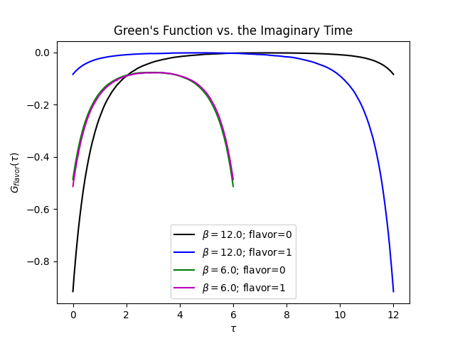
The result shows a Neel transition for the Hubbard model on the Bethe lattice, where the system undergoes a transition from the antiferromagnetic state at low temperatures (“BETA = 12”) to the paramagnetic state at high temperatures (“BETA = 6”).