MC-03 Magnetization

Magnetization curves of quantum spin models

In this tutorial we will look at magnetization curves of quantum spin models using the directed loop SSE application instead of loop, since loop does not perform well in a magnetic field.

One-dimensional Heisenberg chain in a magnetic field

Preparing and running the simulation from the command line

The parameter file parm3a sets up Monte Carlo simulations of the quantum mechanical S=1/2 Heisenberg model on a one-dimensional chain with 20 sites at fixed temperature T=0.08 for a couple of magnetic fields (h=0, 0.1, …, 2.5).

LATTICE="chain lattice" 
MODEL   = "spin"
local_S=1/2
L=20
J=1
T=0.08
THERMALIZATION=2000
SWEEPS=10000
{h=0;}
{h=0.1;}
{h=0.2;}
{h=0.3;}
{h=0.4;}
{h=0.5;}
{h=0.6;}
{h=0.7;}
{h=0.8;}
{h=0.9;}
{h=1.0;}
{h=1.2;}
{h=1.4;}
{h=1.6;}
{h=1.8;}
{h=2.0;}
{h=2.2;}
{h=2.4;}
{h=2.5;}

Using the following standard sequence of commands, you can run the simulation using the quantum SSE code. As usual, XML output files may be viewed in a web browser.

parameter2xml parm3a
dirloop_sse --Tmin 10 --write-xml parm3a.in.xml

Preparing and running the simulation using Python

Setting up and running the simulation in Python is as before, with the script tutorial3a.py:

import pyalps
import matplotlib.pyplot as plt
import pyalps.plot

parms = []
for h in [0., 0.1, 0.2, 0.3, 0.4, 0.5, 0.6, 0.7, 0.8, 0.9, 1.0, 1.2, 1.4, 1.6, 1.8, 2.0, 2.2, 2.4, 2.5]:
    parms.append(
    { 
        'LATTICE'        : "chain lattice", 
        'MODEL'          : "spin",
        'local_S'        : 0.5,
        'T'              : 0.08,
        'J'              : 1 ,
        'THERMALIZATION' : 1000,
        'SWEEPS'         : 20000,
        'L'              : 20,
        'h'              : h
    }
)

input_file = pyalps.writeInputFiles('parm3a',parms)
res = pyalps.runApplication('dirloop_sse',input_file,Tmin=5)

We now have the same output files as in the command line version.

Evaluating the simulation and preparing plots using Python

To load the results and prepare plots we load the results from the output files and collect the magntization density as a function of magnetic field from all output files starting with parm3a.

data = pyalps.loadMeasurements(pyalps.getResultFiles(prefix='parm3a'),'Magnetization Density')
magnetization = pyalps.collectXY(data,x='h',y='Magnetization Density')

To make plots we call the pyalps.pyplot.plot and then set some nice labels, a title, and a range of y-values:

plt.figure()
pyalps.plot.plot(magnetization)
plt.xlabel('Field $h$')
plt.ylabel('Magnetization $m$')
plt.ylim(0.0,0.5)
plt.title('Quantum Heisenberg chain')
plt.show()

One-dimensional Heisenberg ladder in a magnetic field

The parameter file parm3b sets up Monte Carlo simulations of the quantum mechanical S=1/2 Heisenberg model on a one-dimensional ladder with 40 sites at fixed temperature T=0.08 for a couple of magnetic fields (h=0, 0.1, …, 3.5).

LATTICE="ladder" 
MODEL   = "spin"
LATTICE_LIBRARY="../lattices.xml" 
MODEL_LIBRARY="../models.xml"
local_S=1/2
L=20
J0=1
J1=1
T=0.08
...

The rest of the input file is as above and simulations are run in the same way. The corresponding script is downloadable here.

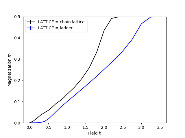
Combining all simulations

The procedure to combine all results into one plot after running both simulations is extremely similar to the previous tutorial. The script is downloadable here. Here is the combined plot:

(missing picture)

Questions

• How does the magnetization depend on the magnetic field?
• How does the magnetization depend on the lattice?
• Bonus: You can also study a 3-leg, 4-leg ladder by changing the parameter W for the width or a spin-1, spin-3/2 chain by changing the parameter local_S. Is there a systematic behavior?